August 2026
Hi all! The Northern Hemisphere summer has come and gone, and with relatively little fanfare in the Arctic this year. That doesn’t mean there were not areas of climate extremes or that the long-term climate change trends have suddenly reversed, but rather that there wasn’t quite as much to talk about as in some previous years (in the news). For understandable reasons, most of the media attention has been on the record warm oceans (ICYMI, we are now over 100 consecutive days of new daily record sea surface temperatures globally) and El Niño, which is alarming but has also had its share of very poor science communication examples, including plenty of misleading data interpretations (and we are only getting started, yikes!). This blog will recap a bit about this past summer across the Arctic.
I also want to share some exciting news that I’ll be traveling to Churchill, Canada in late October to visit Polar Bears International and do some science communication around the impacts of our rapidly changing Arctic. I’ll be sure to post pictures and share a bit more about my experience. This is my first time back to the far north since my trip on an icebreaker north of Svalbard in graduate school, so I am extremely excited! Hopefully I get a chance to visit Alaska someday too.
Anyways, another summer goes by without any new Arctic sea-ice extent records. My featured visualization for this blog shows daily Arctic sea-ice concentration from 15 April 2026 to 12 September 2026 using a high-resolution algorithm (approximately 3 km grid) from the AMSR2 satellite instrument. Note that there are some satellite-related artifacts along coastal regions that occasionally return false positive sea-ice pixels, but you can mostly ignore them. I intentionally made the video animation speed really fast (though you can change that in the settings) so that you can see how changes in weather affect patterns of ice movement and melt. This is common every summer. As a reminder, sea ice follows a seasonal cycle, growing through the winter to reach its maximum extent in March and melting through the summer to reach its minimum in September. The visualization shows the main story of this summer, which I will talk about in more detail below: the early melt-out on the Atlantic side of the Arctic and the slow melt season on the Pacific side. It was really quite a striking dipole pattern of sea-ice concentration anomalies, particularly in June and July.
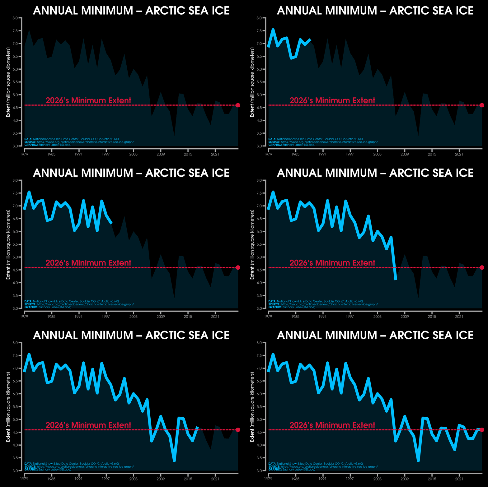
Preliminary satellite data processed by the National Snow and Ice Data Center (NSIDC) show that this year’s annual minimum Arctic sea-ice extent was statistically tied for the 10th lowest on record, along with 2008, 2010, and 2025. For 2026, Arctic sea-ice extent fell to 4.60 million square kilometers (1.78 million square miles), which is approximately 1.62 million square kilometers (625,000 square miles) below the 1981-2010 average. The minimum on September 12th was set 2 days earlier than average. 2012 still holds the all-time record.
The 20 lowest September sea-ice minimums have all been set in the last 20 years, which is the takeaway statistic for describing how the Arctic has changed considerably in the last several decades.
As of writing this blog, daily sea-ice extent is around the 16th lowest on record (for the date), with the freeze season now well underway. The relatively unimpressive ranking after the annual minimum is common when years have highly fragmented ice, like this one. This is because the areas of open water between the sea-ice floes quickly refreeze and rapidly boost sea-ice extent numbers, so I am not that surprised that we are more extensive than the 2010s decadal average for this time of year.
Note that our data is still limited for real-time estimates of sea-ice thickness and volume (missing PIOMAS), but we should get some sea-ice thickness information soon from the new summertime hybrid ICESat-2 and CryoSat-2 products. Although there were no new records for metrics like ice extent, we can see just how fragmented and diffuse the ice cover was this summer. In fact, MODIS satellite imagery showed widespread open water yet again, not far from the North Pole.
As we have learned more and more, local weather patterns across the Arctic play a really important role in year-to-year sea-ice extent variability, even as the long-term trend is clearly downward. In fact, just this winter we observed the lowest sea-ice extent on record for the annual maximum in March. Recent research has shown that slowdowns in the rate of Arctic sea-ice decline are expected due to internal climate variability. This means that although the long-term trend is downward, there can be decades when internal variability acts to further accelerate that decline, or the reverse, contributing to periods with little-to-no trend. There are also other key climate feedbacks at play as the Arctic rapidly changes, such as increased winter ice growth because thinner ice can grow faster. Another factor is probably related to the metric we use to monitor Arctic sea ice most commonly. “Sea-ice extent” can sometimes tally areas with lower sea-ice concentration where the ice is more fragmented and dispersed across the Arctic, even when there are large leads and open areas of water.
Overall, this summer was influenced mainly by lower pressure toward the central Arctic, which brought cloudier and cooler conditions that limited surface melt and delayed the start of the melt season. This was most obvious across parts of the Beaufort and Chukchi Seas, where the melt season didn’t really kick off until after early July, more than two weeks later than normal. In fact, one of the most striking statistics was in the Beaufort Sea, where sea-ice cover through June covered nearly the entire basin and was even as extensive as back in the 1980s. Eventually, the lower-concentration ice gave way to a more rapid melt-out in early August, with sea-ice extent on the Pacific side of the Arctic more closely falling back to below the 1981-2010 average conditions.
In contrast, the Atlantic side of the Arctic had a much more extreme summer. Sea ice in the Barents Sea actually had its earliest melt-out on record, as I wrote about in an earlier blog. This was in part due to unusually warm air and ocean temperatures, as well as winds that helped push the ice northward.
Despite cooler temperatures over the central Arctic Ocean, conditions over surrounding land areas were much more extreme overall this summer. Parts of western Siberia saw unusually persistent temperatures more than 5°C above the 1981-2010 average for much of the last few months, which extended out over the Kara Sea and contributed to substantial ice melt in this area. This is also consistent with the long-term climate change trend, where some of the largest declines in sea-ice cover have occurred in the Barents and Kara Seas regions.
Another area of warmer sea surface temperatures has been in parts of the East Siberian Sea, where there are also correspondingly low sea-ice conditions. The Laptev Sea, on the other hand, has experienced less melt this summer compared to some of the more extreme recent years. Differences across marginal seas of the Arctic Ocean are always an important piece of the Arctic climate story, and the orientation of surface winds can play a big role in why some areas see more extensive ice than others, as winds (and ocean currents) can either spread the ice outward or compact it and push the ice edge poleward.
Overall, this past year across the Arctic Circle has featured some particularly remarkable contrasts in extremes and examples of weather whiplash. There has been no shortage of new climate records, unfortunately, even though this summer’s average ice extent was less anomalous than in some recent summers. For future Arctic sea-ice research, it remains crucial to better understand the connections between year-to-year variability in the large-scale atmospheric circulation across the Arctic and the long-term warming trend from human-caused climate change. Better understanding this variability will give us more insight into when we might see a future ice-free September. I also think it is important to support more data and observations of other sea-ice metrics, like ice thickness/volume, which may give us better insight into the overall condition of the ice pack, especially during years like 2026 when it is very fragmented.
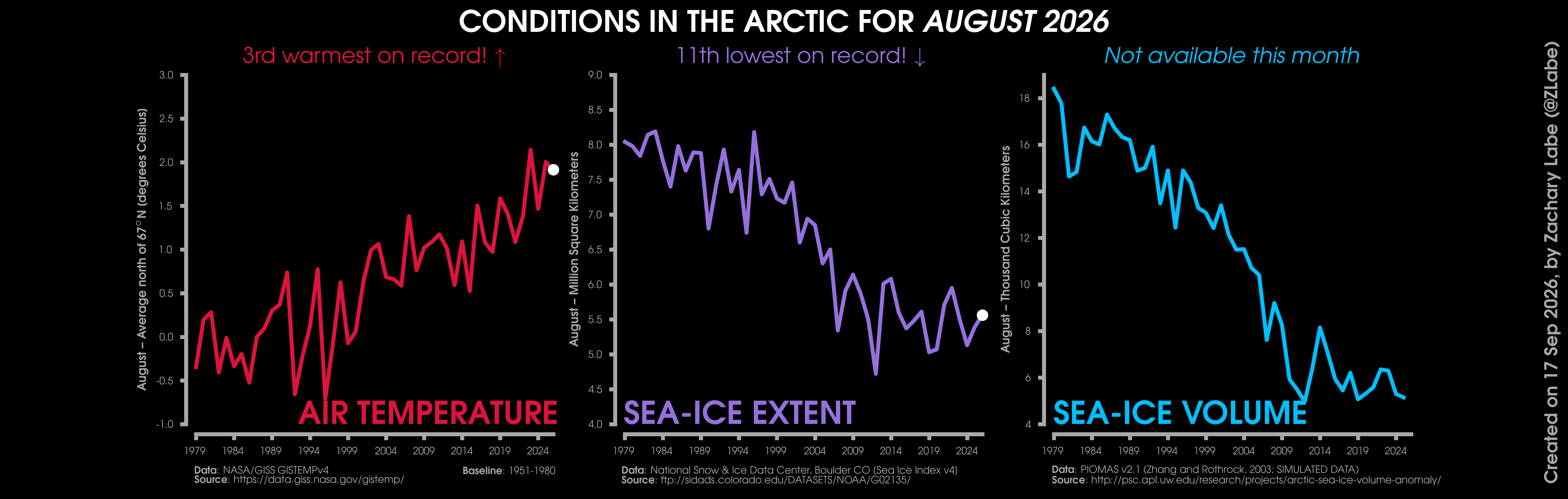
Changes in mean surface air temperature anomalies (GISTEMPv4; 1951-1980 baseline), mean Arctic sea ice extent (NSIDC; Sea Ice Index v4), and mean Arctic sea ice volume (PIOMAS v2.1; Zhang and Rothrock, 2003) over the satellite era. Updated 9/17/2026.
Finally, looking at my August Arctic dashboard shows a similar theme to this past summer, with relatively warm conditions (ranking 3rd warmest using NASA GISTEMPv4) but more extensive ice compared to some past years. Sea-ice concentration anomalies were largest over the northern Barents-Kara Seas region, as well as parts of the East Siberian Sea. Like most of the summer, temperature departures were largest over western Siberia, with relatively cooler conditions for latitudes north of 80°N.
To answer some questions, it is unlikely that El Niño is having any major tangible effects on the Arctic right now, and its overall connections to the region are a lot less clear than for other parts of the world. It is important to keep in mind that although El Niño is associated with a temporary boost in global mean temperatures, that doesn’t mean it brings heat everywhere. In fact, a lot of the reason for that boost is because many of the warmer temperature anomalies are concentrated across the Tropics in association with El Niño (and of course some other areas, like western North America). Because of this, along with the mixed results in the research literature and via some simple lead-lag correlation analysis, I have no predictions on how this El Niño may or may not affect regional weather in the Arctic (especially given the concurrent negative phase of the Pacific Decadal Oscillation). But I will certainly keep you all updated.
Thank you for reading! My other monthly blogs since 2022 are linked below. If you’d like to support the effort behind maintaining and updating these website graphics, you can do so here: https://buymeacoffee.com/zacklabe. Last thing I will mention is that I am now on Threads too for social media posts, as I continue to try expanding my audience for sharing this important climate information.
Other Blogs (Monthly):

Other Climate Data Statistics (Monthly):
My Visualizations:
My research related to data visualization:
[2] Witt, J.K., Z.M. Labe, A.C. Warden, and B.A. Clegg (2023). Visualizing uncertainty in hurricane forecasts with animated risk trajectories. Weather, Climate, and Society, DOI:10.1175/WCAS-D-21-0173.1
[HTML][BibTeX][Code]
[Blog][Plain Language Summary][CNN]
[1] Witt, J.K., Z.M. Labe, and B.A. Clegg (2022). Comparisons of perceptions of risk for visualizations using animated risk trajectories versus cones of uncertainty. Proceedings of the Human Factors and Ergonomics Society Annual Meeting, DOI:10.1177/1071181322661308
[HTML][BibTeX][Code]
[Plain Language Summary][CNN]
The views presented here only reflect my own. These figures may be freely distributed (with credit). Information about the data can be found on my references page and methods page.