Hi! My name is Zack! I’m a climate scientist looking to find the signal in all the noise. I use data-driven methods to untangle climate change patterns from natural variability, providing clearer insights into climate risks. I also spend a lot of time thinking about how to make science more engaging through storytelling and visualization.
Heatmap-style visualization showing global average surface temperature anomalies, which are calculated relative to pre-industrial levels (1850-1900 – outlined in the IPCC Special Report on Global Warming of 1.5°C). Data is from NOAA Merged Land Ocean Global Surface Temperature Analysis (NOAAGlobalTemp v6.1.0; https://www.ncei.noaa.gov/products/land-based-station/noaa-global-temp). Graphic updated using data through February 2026. Red dots mark the year of each respective warmest month in this dataset.
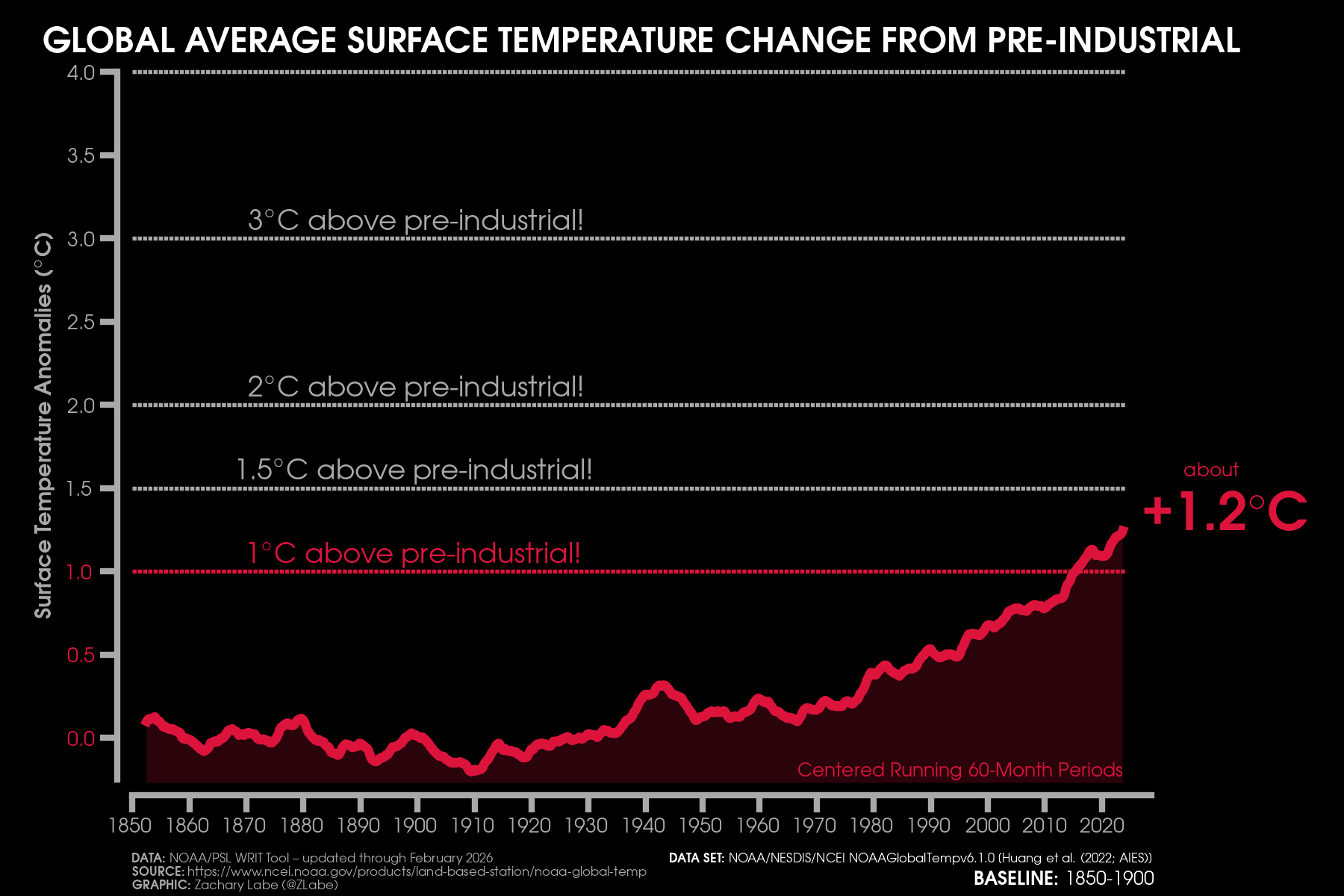
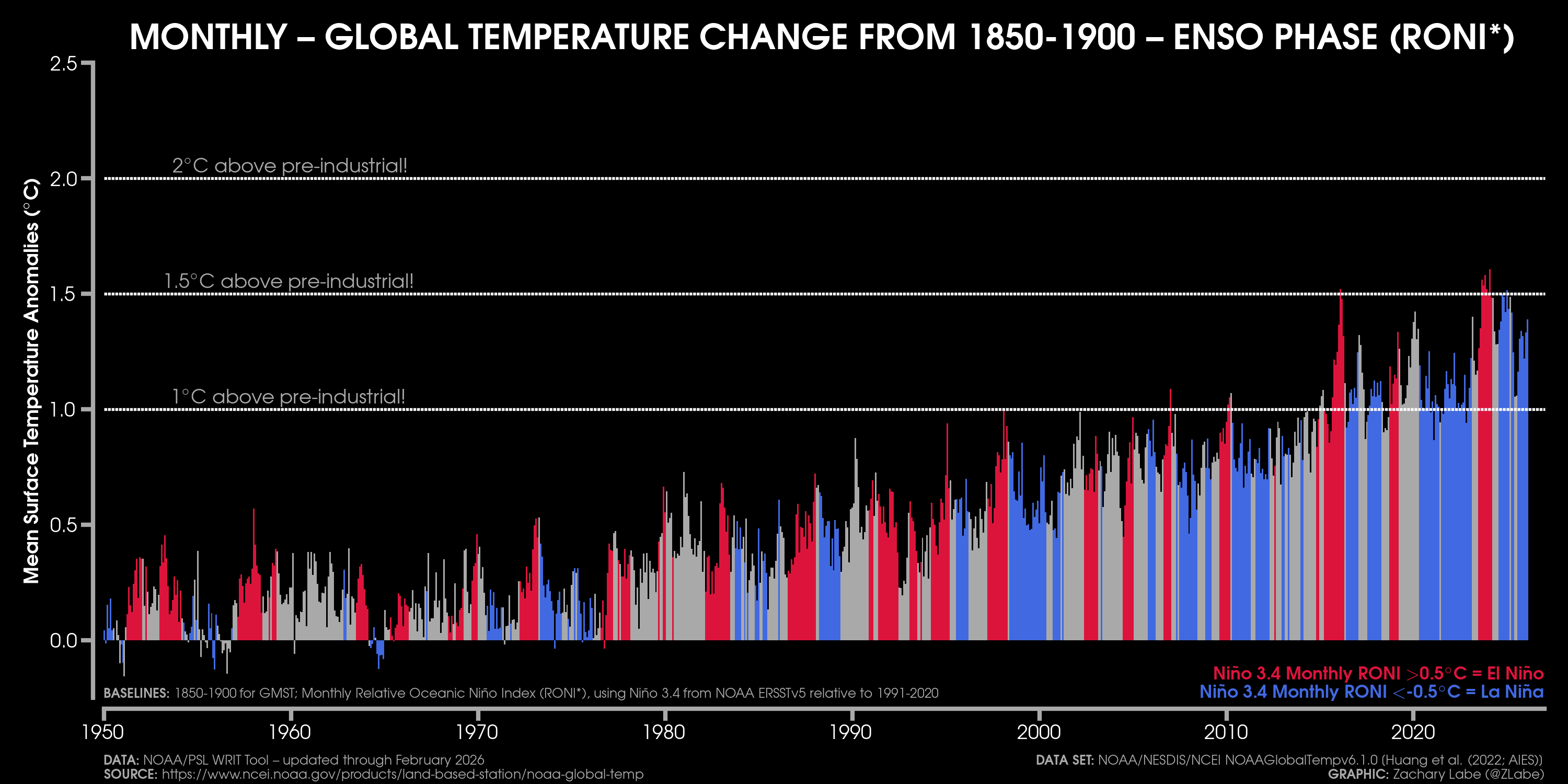
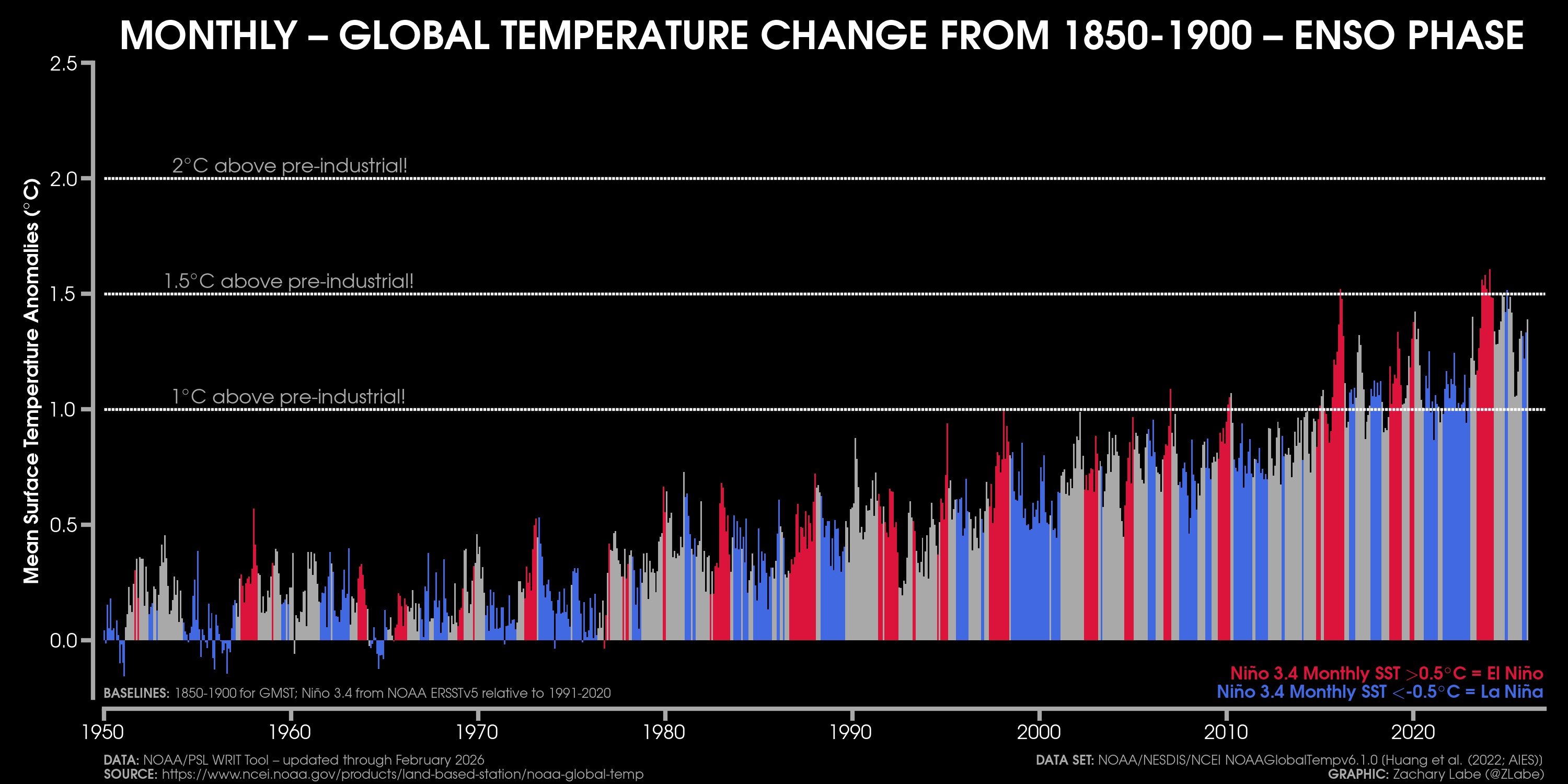
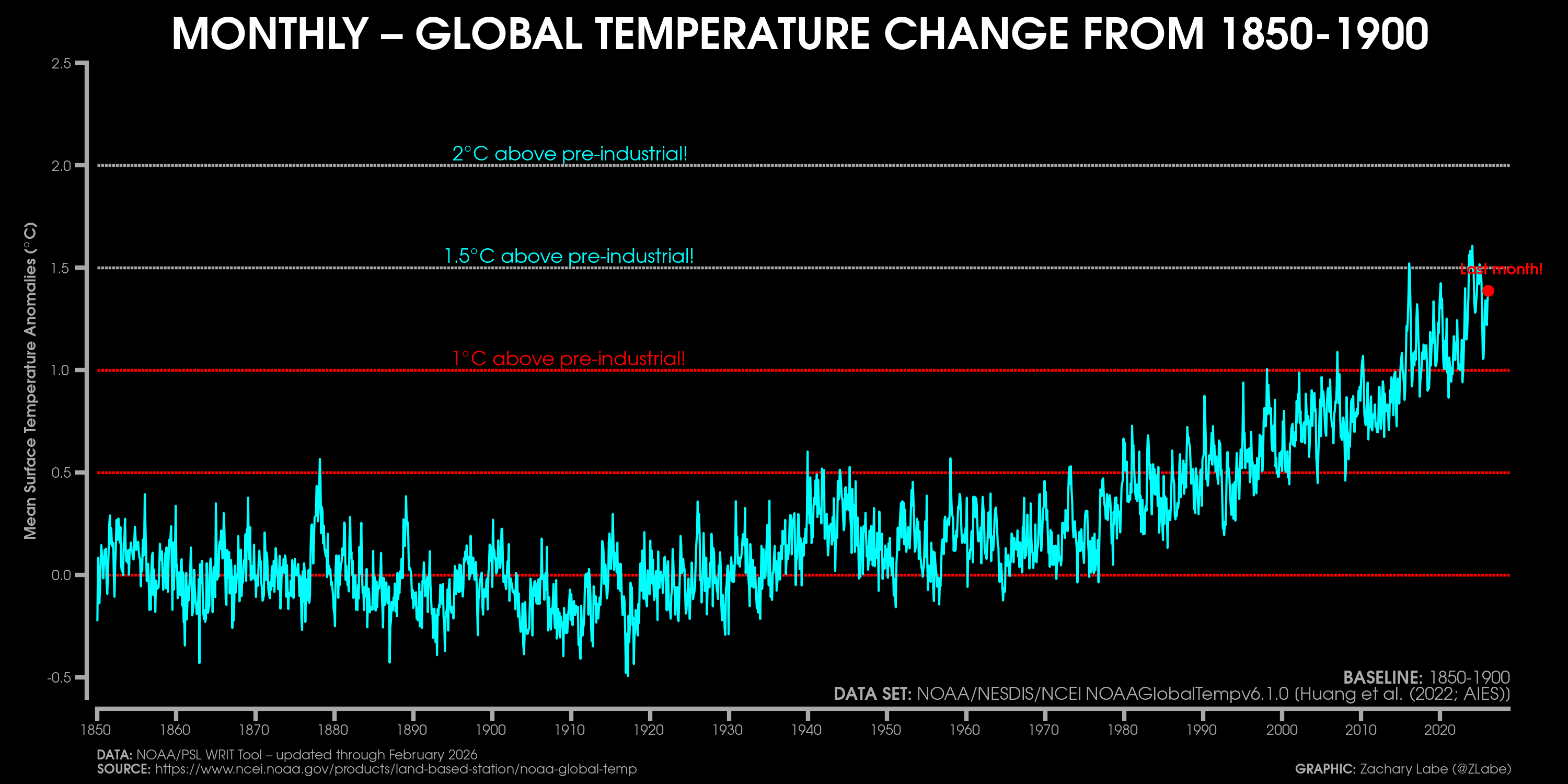
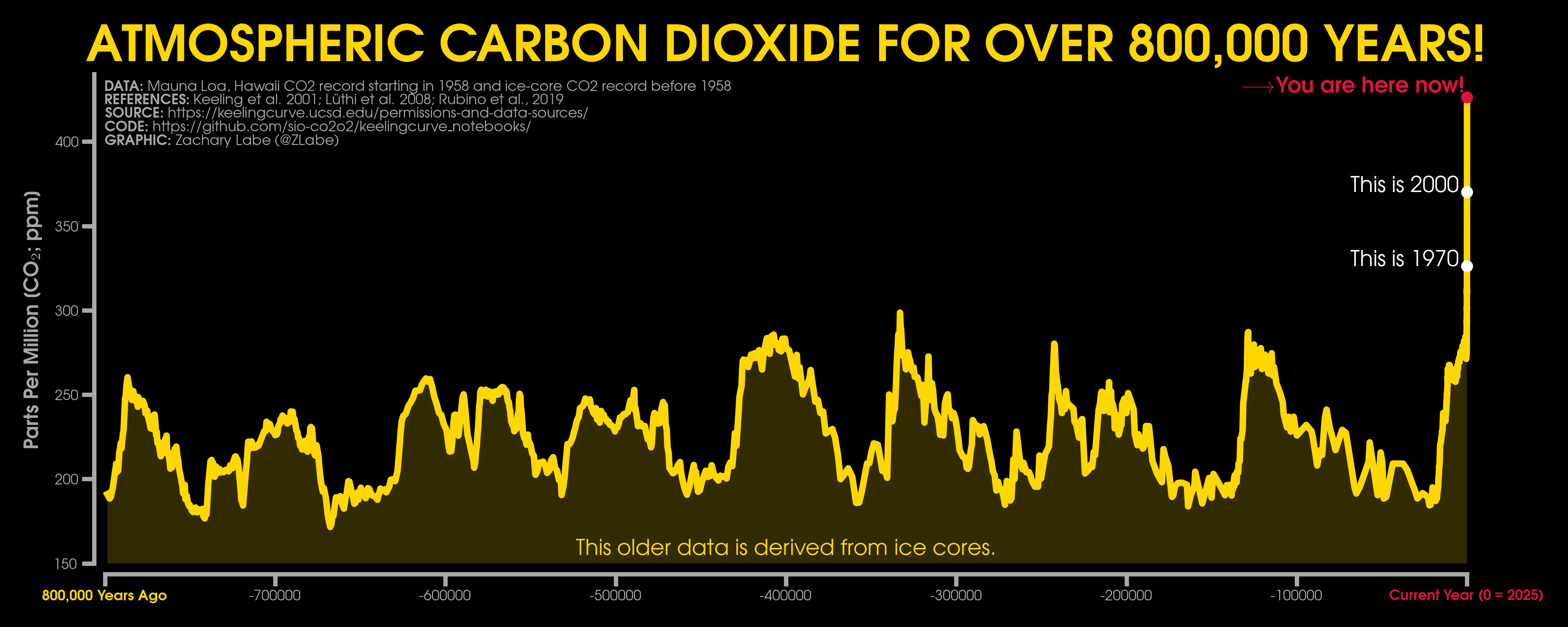
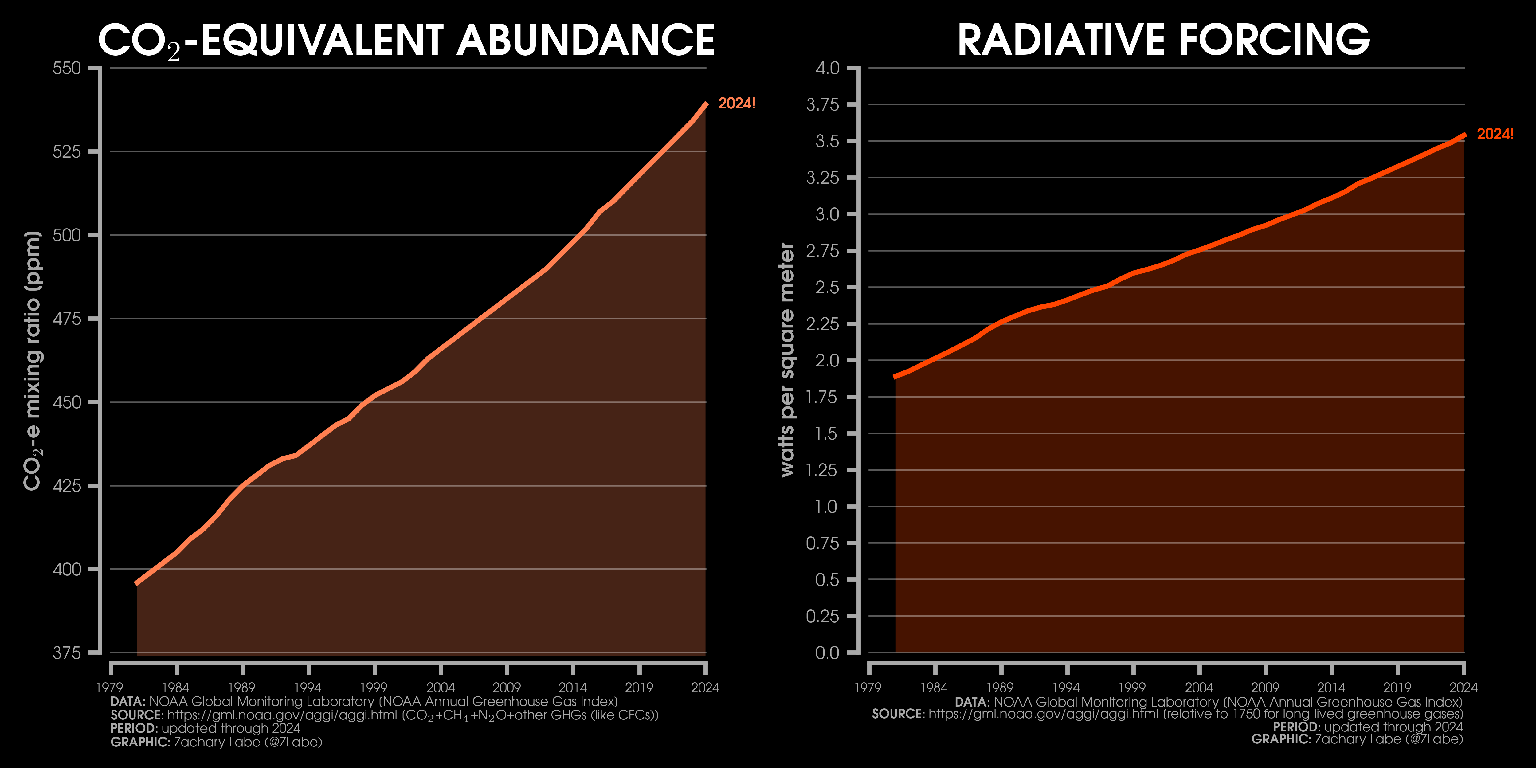
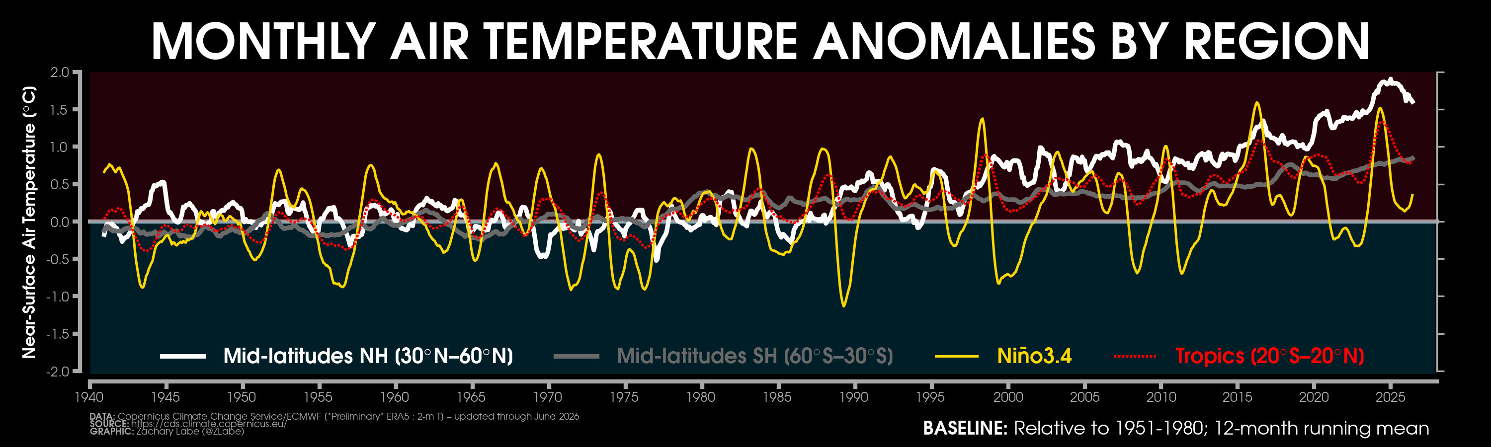
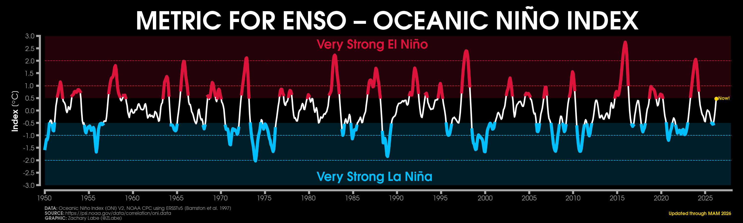
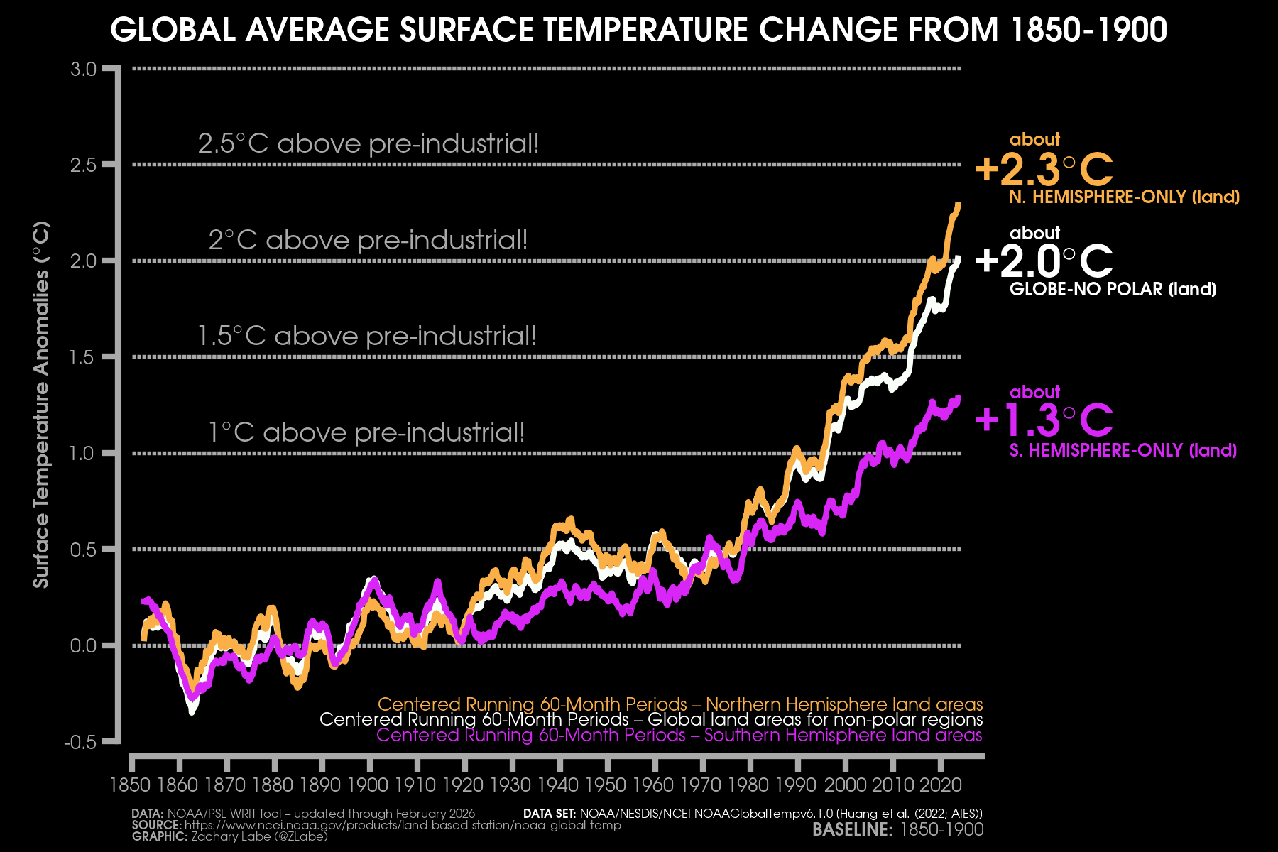
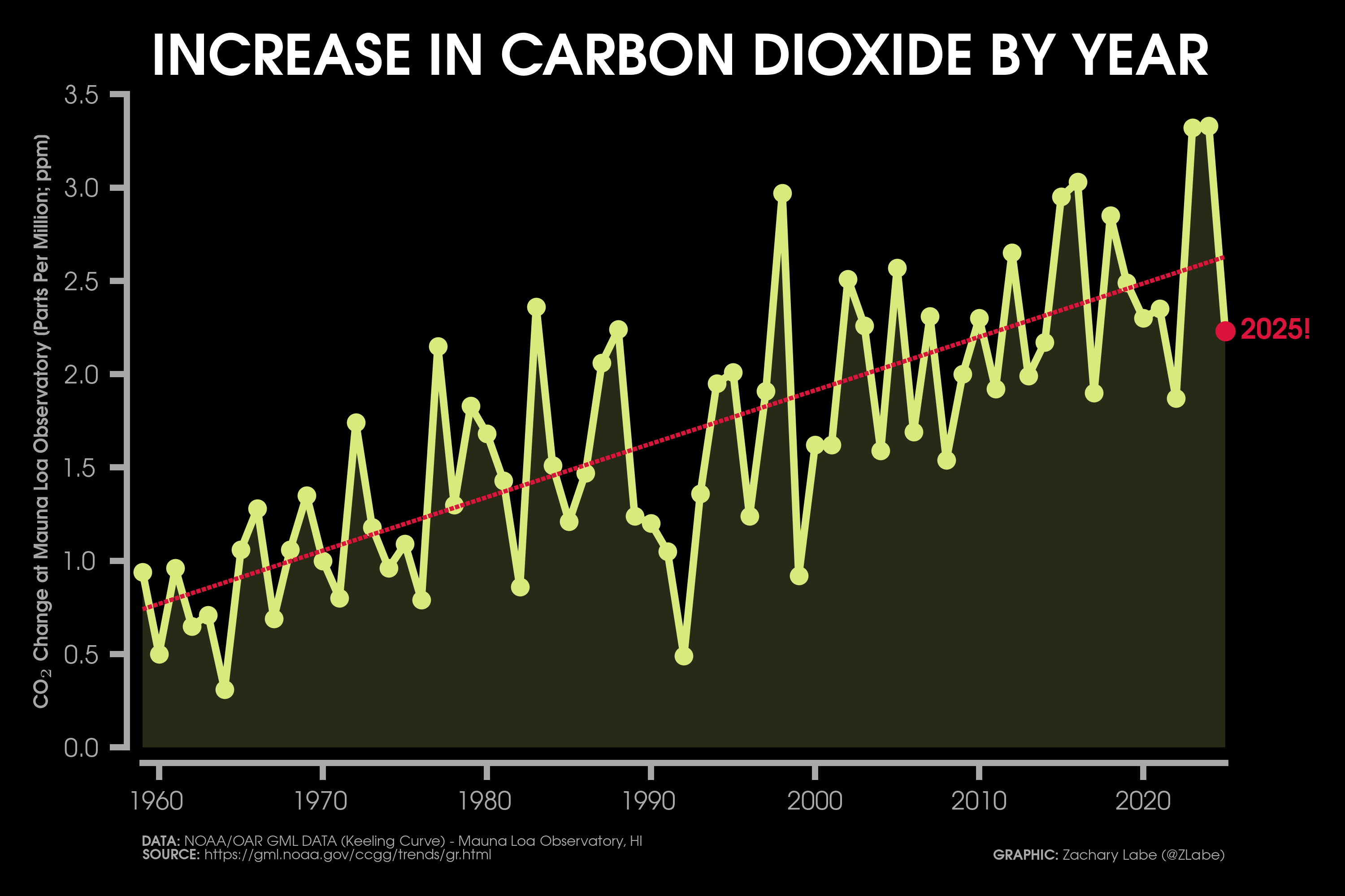
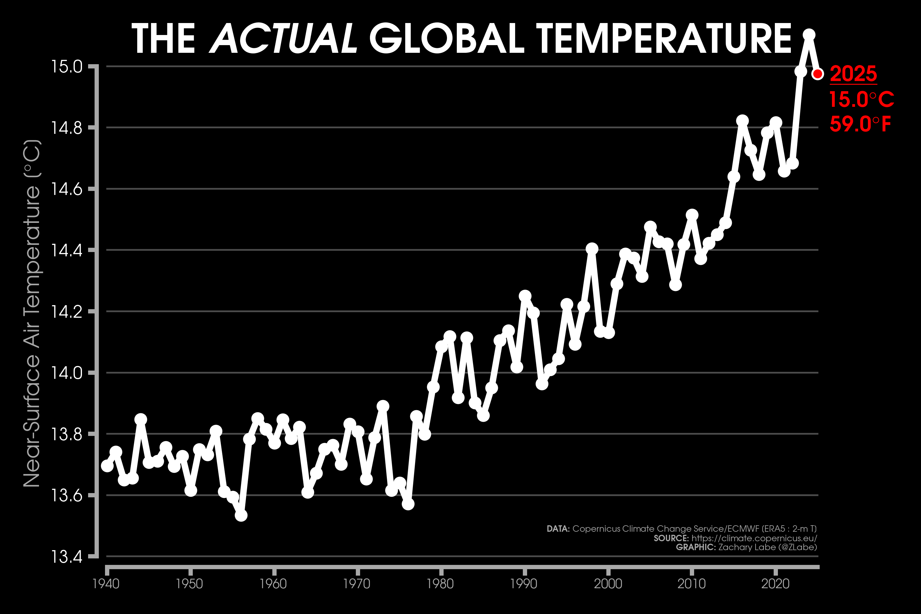
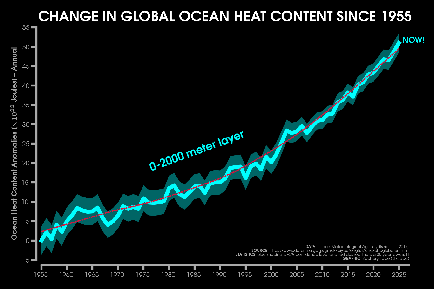
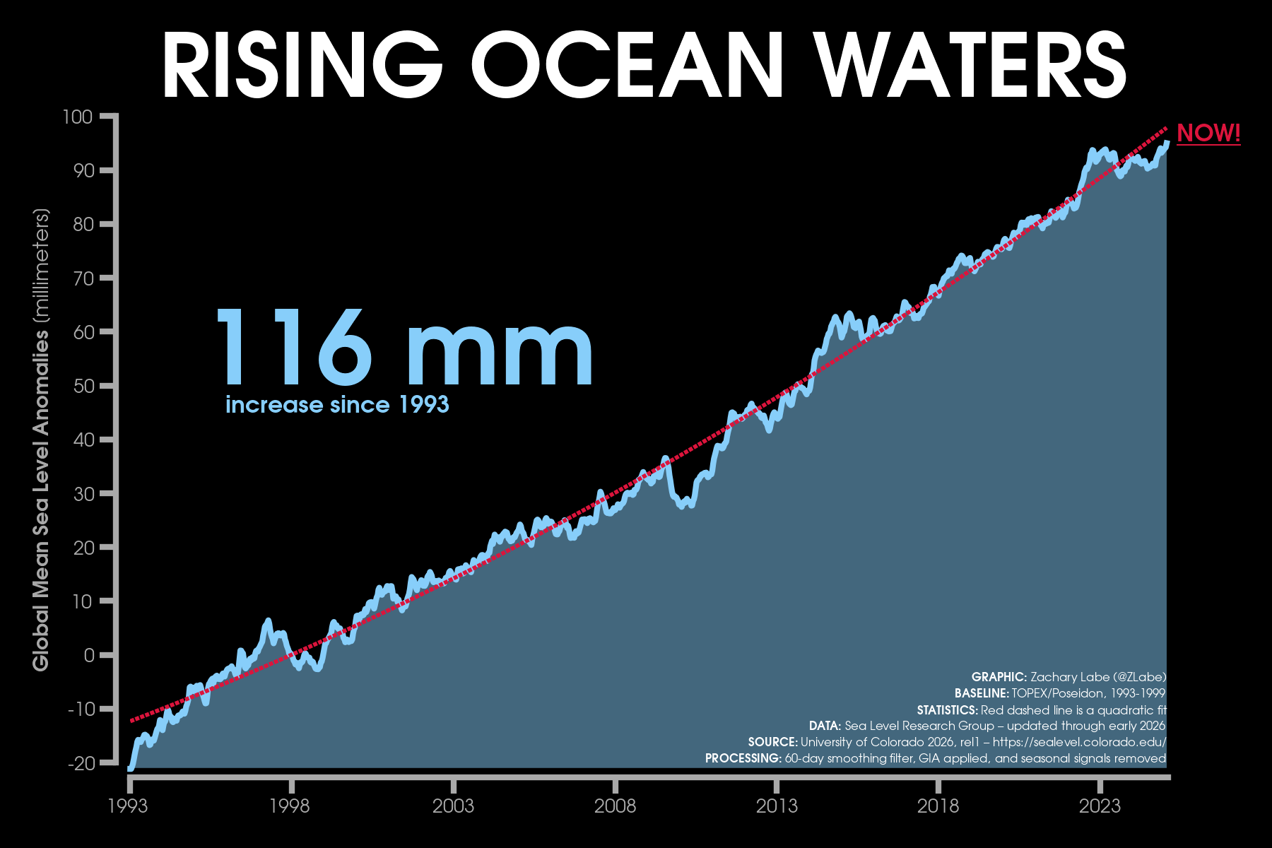
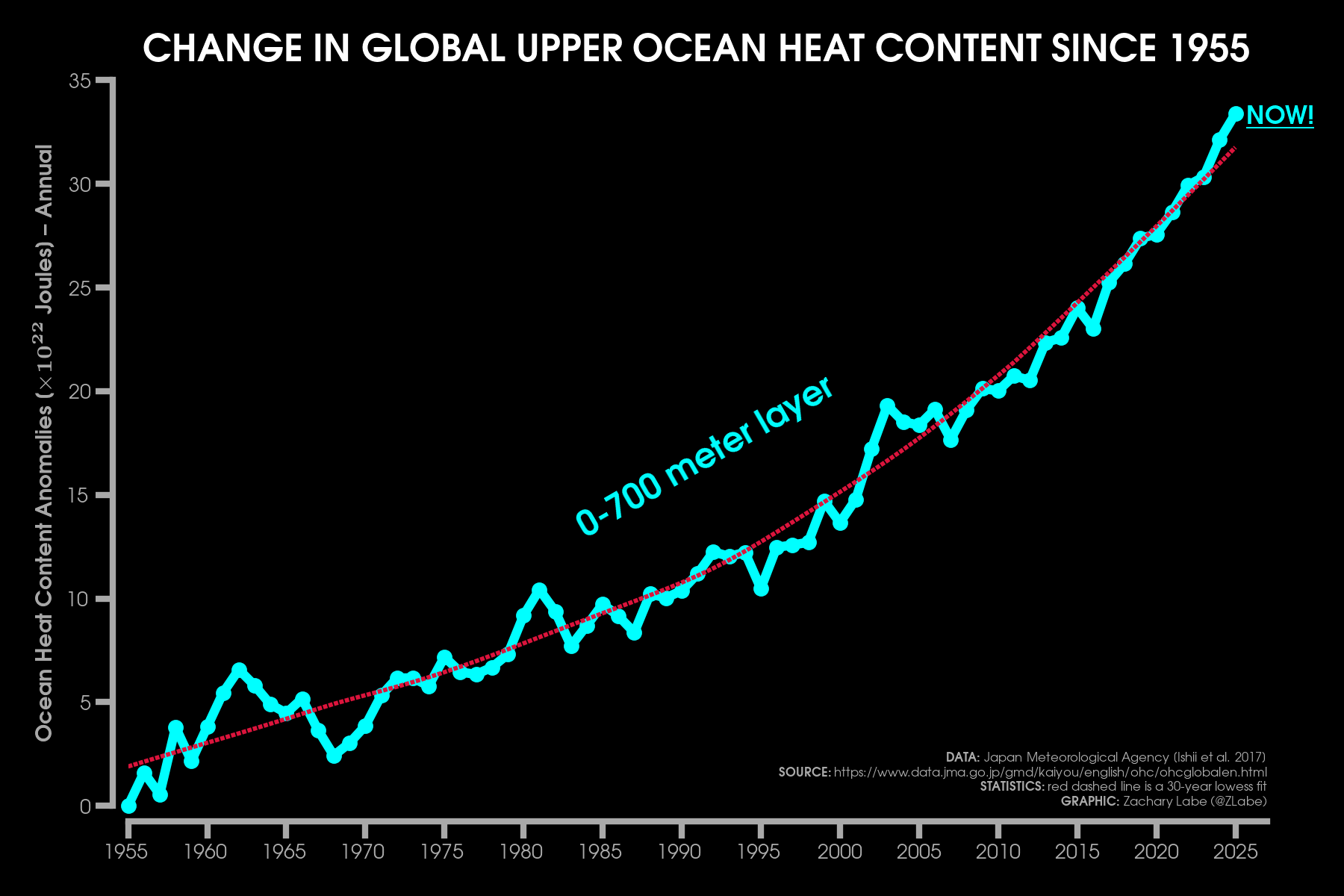
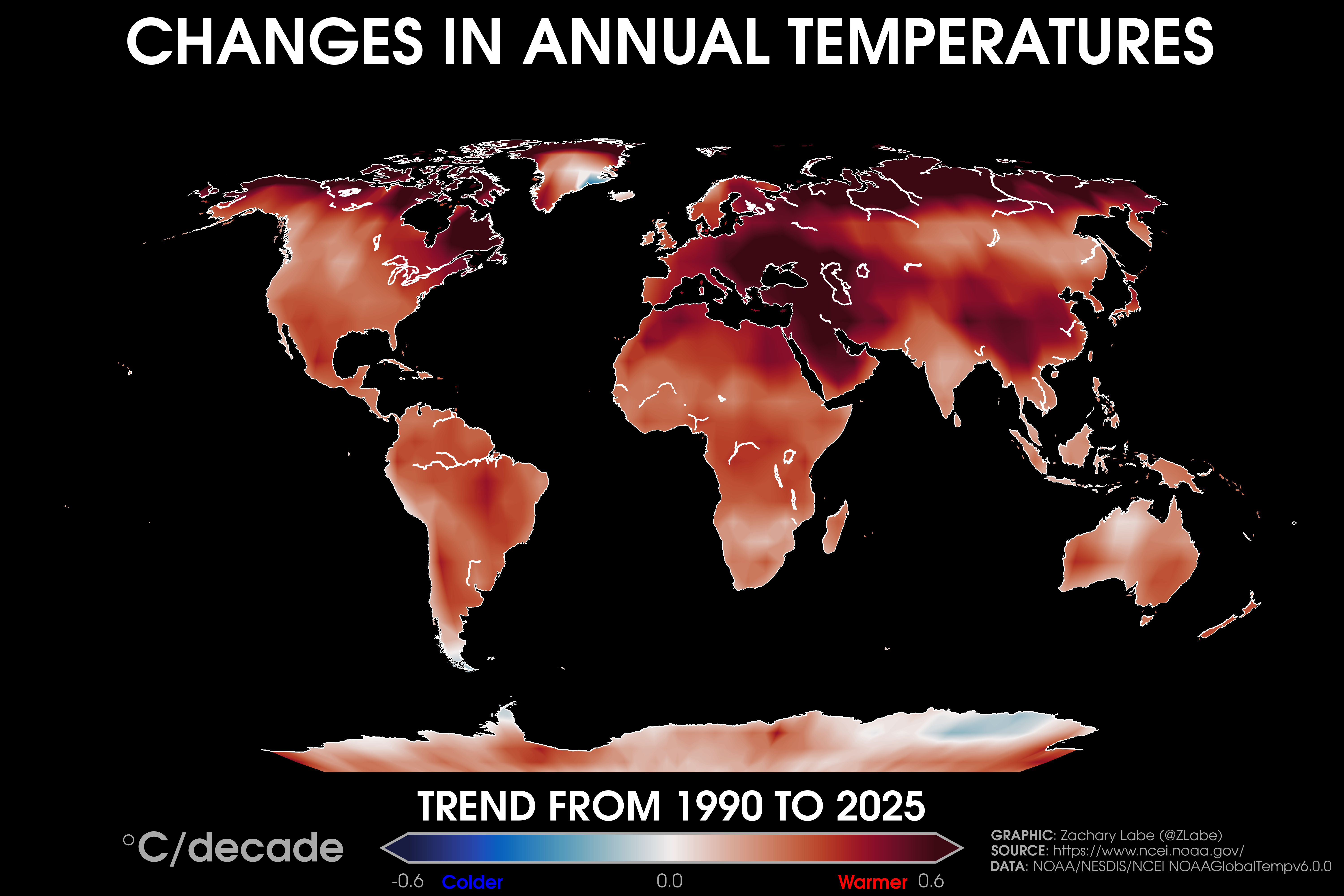
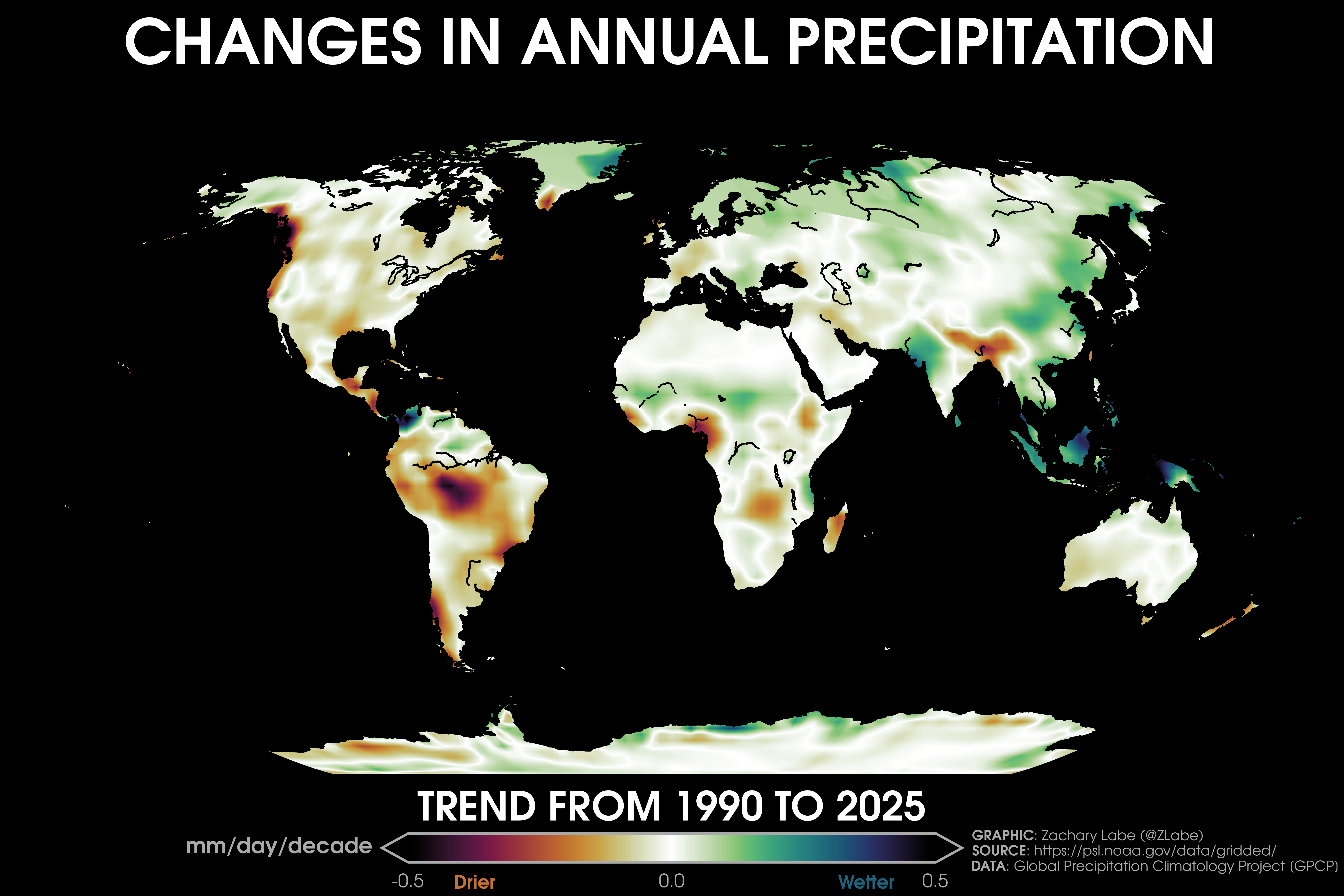
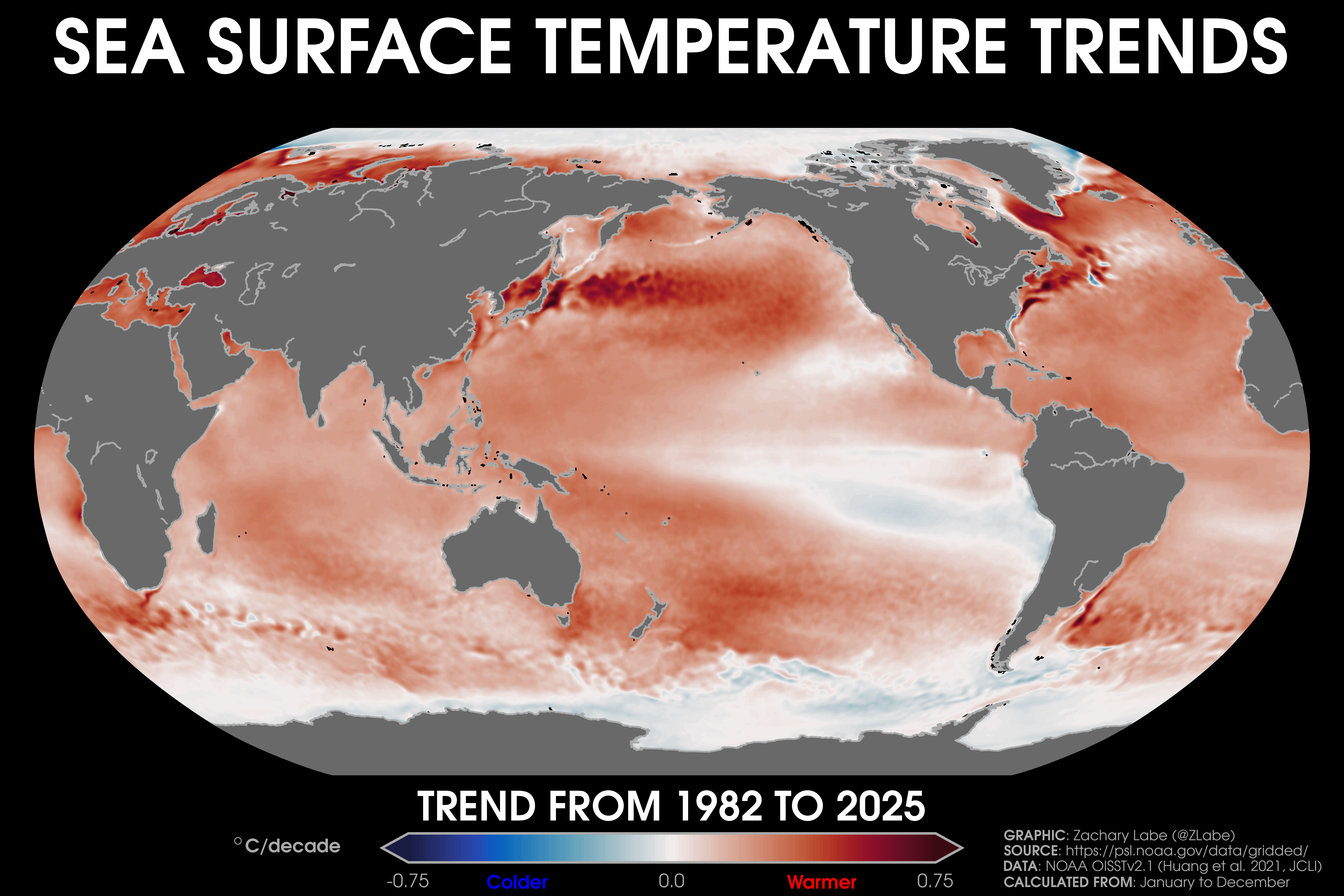
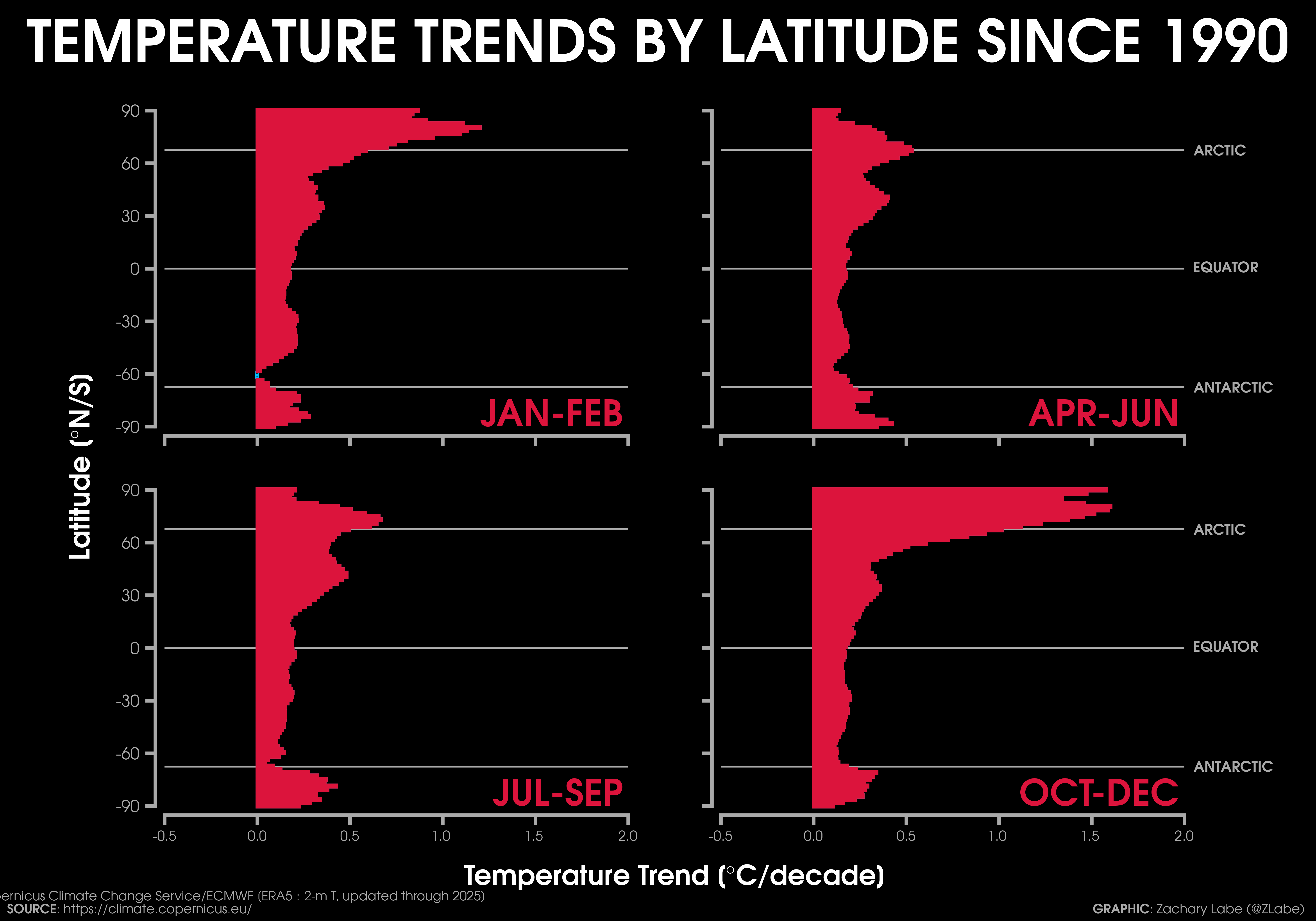
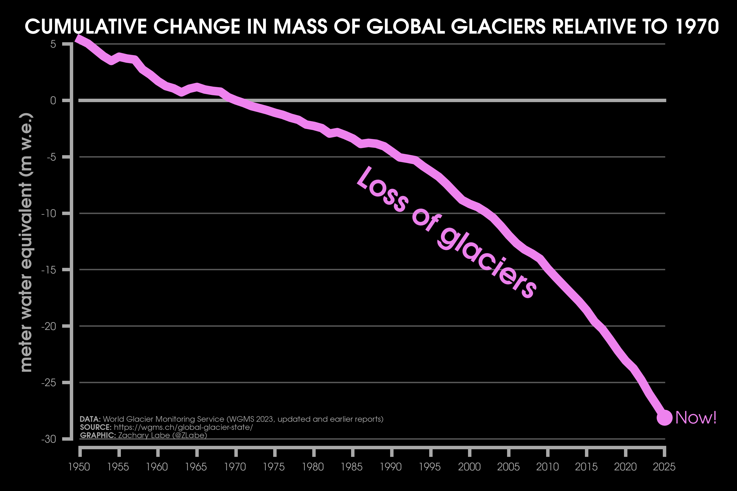
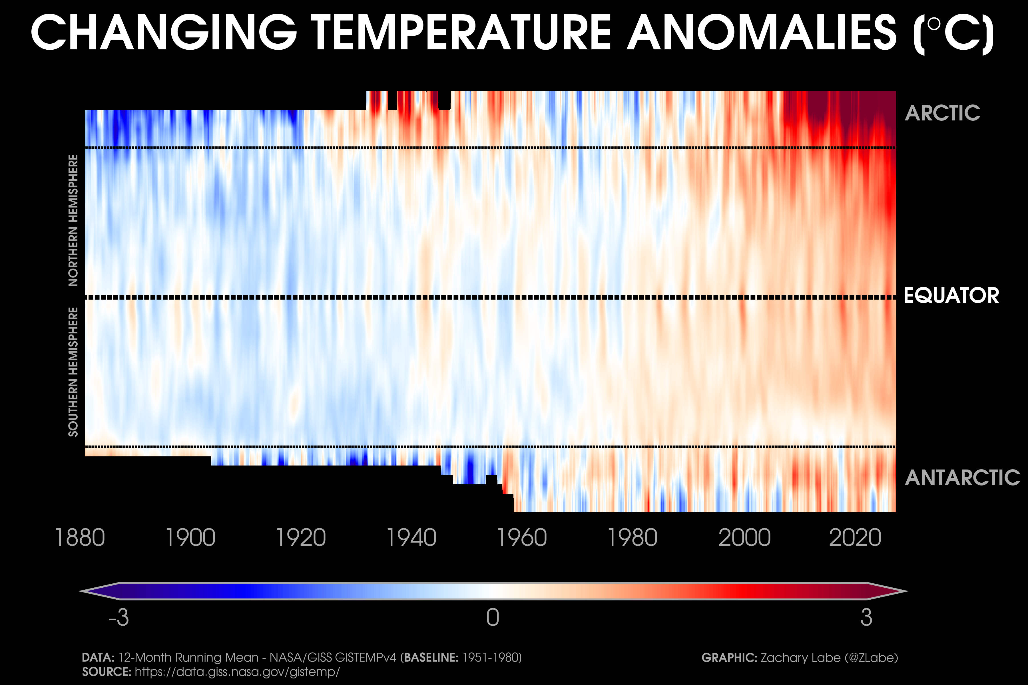
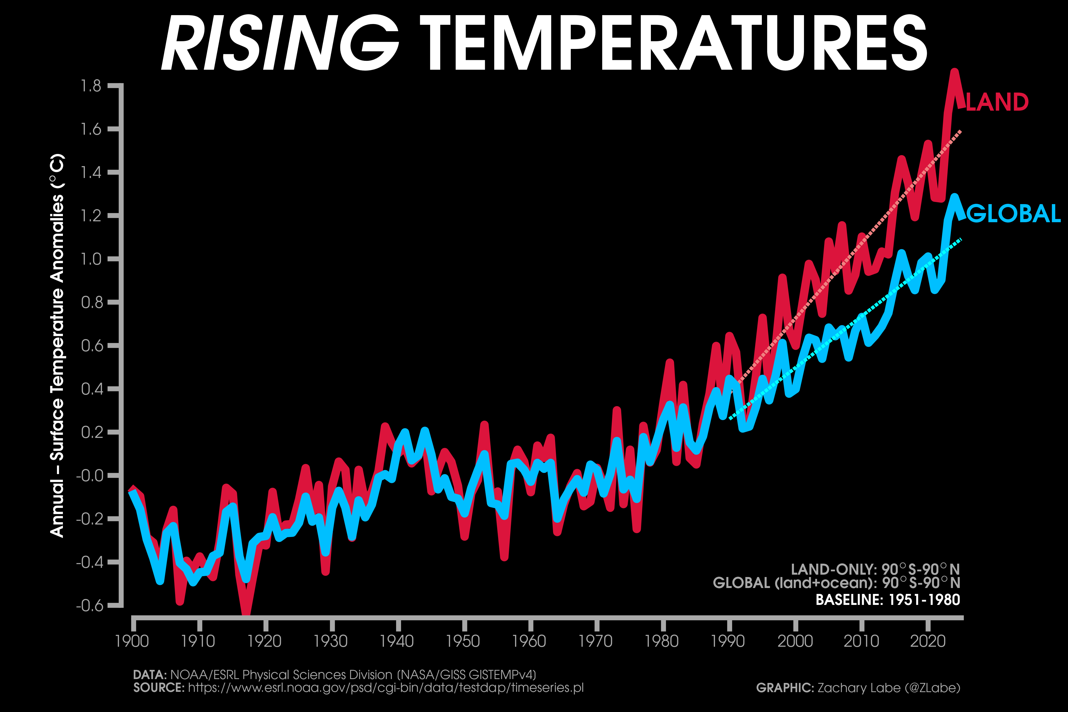
Daily global mean near-surface (2-m) air temperatures using ECMWF ERA5 reanalysis (area-weighted average). The spread in the years 1940-2025 are annotated by the gray shading. 2026 is shown with the red line. 2024 is shown with a thin white line. Climatological reference periods are shown with dashed dark green, light green, and while lines for the respective 30-year baselines of 1971-2000, 1981-2010, and 1991-2020. A dashed dark red line indicates 2°C above the 1850-1900 pre-industrial baseline, as defined by C3S (https://climate.copernicus.eu/GCH2023-Paris-Agreement). Due to preliminary data from ERA5T (for 2026), this graphic will be updated at a 2-3 day lag. Data are provided by https://pulse.climate.copernicus.eu/. The graphic is updated through 6 July 2026.Daily global mean sea surface temperatures (SST) using ECMWF ERA5 reanalysis (area-weighted average from 60°S to 60°N). The spread in the years 1979-2025 are annotated by the gray shading. 2026 is shown with the red line. 2024 is shown with a thin white line, and 2023 is shown with a thin orange line. Climatological reference periods are shown with dashed light green and while lines for the respective 30-year baselines of 1981-2010 and 1991-2020. Due to preliminary data from ERA5T (for 2026), this graphic will be updated at a 2-3 day lag. Data are provided by https://pulse.climate.copernicus.eu/. The graphic is updated through 6 July 2026.Monthly global mean near-surface (2-m) air temperatures using ERA5 reanalysis (area-weighted average). Individual years from 1940-2025 are shown by the sequential purple to white lines. 2026 is indicated by the red line, and 2024 is shown with a yellow line. Due to preliminary data from ERA5T (for 2026), this graphic will be updated at a 1-month lag. Updated through June 2026Global average surface temperature anomalies for centered running 60-month periods. Monthly anomalies are calculated relative to pre-industrial levels (1850-1900 – outlined in the IPCC Special Report on Global Warming of 1.5°C). Data is from NOAA Merged Land Ocean Global Surface Temperature Analysis (NOAAGlobalTemp v6.1.0; https://www.ncei.noaa.gov/products/land-based-station/noaa-global-temp). Graphic updated using data through February 2026.Bar graph showing monthly global average surface temperature anomalies, which are calculated relative to pre-industrial levels (1850-1900 – outlined in the IPCC Special Report on Global Warming of 1.5°C) from 1950 through 2026. Data is from the NOAA Merged Land Ocean Global Surface Temperature Analysis (NOAAGlobalTemp v6.1.0; https://www.ncei.noaa.gov/products/land-based-station/noaa-global-temp). Each bar is shaded by the current phase of the El Niño-Southern Oscillation (ENSO). Months with the Relative Oceanic Niño Index (RONI) above 0.5°C are shaded red (El Niño), and months with the RONI anomaly below -0.5°C are shaded blue (La Niña). Gray bars indicate neutral ENSO conditions. Graphic updated using data through January 2026.Bar graph showing monthly global average surface temperature anomalies, which are calculated relative to pre-industrial levels (1850-1900 – outlined in the IPCC Special Report on Global Warming of 1.5°C) from 1950 through 2026. Data is from the NOAA Merged Land Ocean Global Surface Temperature Analysis (NOAAGlobalTemp v6.1.0; https://www.ncei.noaa.gov/products/land-based-station/noaa-global-temp). Each bar is shaded by the current phase of the El Niño-Southern Oscillation (ENSO). Months with the Niño3.4 sea surface temperature (SST) anomaly (relative to 1991-2020) above 0.5°C are shaded red (El Niño), and months with the Niño3.4 SST anomaly below -0.5°C are shaded blue (La Niña). Gray bars indicate neutral ENSO conditions. Graphic updated using data through January 2026.Monthly global average surface temperature anomalies, which are calculated relative to pre-industrial levels (1850-1900 – outlined in the IPCC Special Report on Global Warming of 1.5°C). Data is from NOAA Merged Land Ocean Global Surface Temperature Analysis (NOAAGlobalTemp v6.1.0; https://www.ncei.noaa.gov/products/land-based-station/noaa-global-temp). Graphic updated using data through February 2026. Monthly temperature anomalies are now consistently at least 1°C above pre-industrial levels, which is why the annotation color is turned from blue to red.Carbon dioxide levels over the last 800,000 years, which are merged from ice cores (https://www.nature.com/articles/nature06949; https://data.csiro.au/collection/csiro:37077) and recent Mauna Loa observations (starting in 1958 through the year 2025). Graphic updated on 1/6/2026Graphic showing CO2-equivalent (CO2-e) atmospheric abundance (left) and radiative forcing (right) from 1979 to 2024 using data from https://gml.noaa.gov/aggi/aggi.html. CO2-e is the amount of carbon dioxide that would be needed to be equivalent to the average radiative forcing from all of the greenhouse gases combined. The direct radiative forcing is calculated for nearly all greenhouse gases relative to a 1750 baseline period. Radiative forcing is a measure of the perturbation (warming) to the climate system from greenhouse gases (i.e., Earth’s energy imbalance in the atmosphere). Graphic was updated on 1/4/2026.Monthly near-surface air temperature anomalies averaged over the Northern Hemisphere (yellow line) and Southern Hemisphere (dashed blue line) from January 1940 to June 2026 (ERA5 reanalysis). Anomalies are calculated from a climatological baseline of 1951-1980 (updated 7/7/2026).Monthly near-surface air temperature anomalies averaged over the Northern Hemisphere mid-latitude region (white line; 30°N-60°N), Southern Hemisphere mid-latitude region (grey line; 60°S-30°S), Niño 3.4 region (yellow line; 120°W-150°W and 5°S-5°N), and the Tropics (dashed red line; 20°S to 20°N) from January 1940 to June 2026 (ERA5 reanalysis). Anomalies are calculated from a climatological baseline of 1951-1980. Data are smoothed using a 12-month forward running average. Graphic updated on 7/7/2026.Monthly near-surface air temperature anomalies averaged over the Arctic (gold line; 65°N-90°N), high Arctic (dashed gold line; 80°N-90°N), Antarctic (blue line; 90°S-65°S), and high Antarctic (blue line; 90°S-80°S) from January 1940 to June 2026 (ERA5 reanalysis). Anomalies are calculated from a climatological baseline of 1951-1980. Data are smoothed using a 12-month forward running average. Graphic updated on 7/7/2026.Time series of the Relative Oceanic Niño Index (RONI; L’Heureux et al. 2024, JCLI), which a metric that uses a 3-month running mean of NOAA ERSSTv5 sea surface temperature anomalies in the Niño 3.4 region. It is similar to the standard ONI, but the RONI accounts for long-term climate warming by subtracting the average sea surface temperature of the entire tropics. This metric is used for monitoring current El Niño-Southern Oscillation (ENSO) conditions in a warming world. Data is available at https://www.cpc.ncep.noaa.gov/data/indices/RONI.ascii.txt. Graphic updated through April-May-June (AMJ) 2026.Time series of the NOAA/CPC Oceanic Niño Index (ONI; Bamston et al. 1997), which uses a 3-month running mean of NOAA ERSSTv5 sea surface temperature anomalies in the Niño 3.4 region. This metric is used for monitoring current El Niño-Southern Oscillation (ENSO) conditions, and more information is available at https://origin.cpc.ncep.noaa.gov/products/analysis_monitoring/ensostuff/ONI_v5.php. Graphic updated through March-April-May (MAM) 2026.Decadal trends in annual mean surface air temperatures over land areas from 1900 to 2025, 1940 to 2025, 1980 to 2025, and 2000 to 2025. Data are from NOAAGlobalTemp v6.0.0 (https://www.ncei.noaa.gov/products/land-based-station/noaa-global-temp). Graphic was updated on 1/17/2026.Global average surface temperature anomalies for centered running 60-month periods (white line) compared to global average surface temperature anomalies over only land areas for centered running 60-month periods (red line). Monthly anomalies are calculated relative to pre-industrial levels (1850-1900 – outlined in the IPCC Special Report on Global Warming of 1.5°C). Data is from NOAA Merged Land Ocean Global Surface Temperature Analysis (NOAAGlobalTemp v6.1.0; https://www.ncei.noaa.gov/products/land-based-station/noaa-global-temp). Graphic updated using data through February 2026.Global average surface temperature anomalies for centered running 60-month periods (white line) compared to global average surface temperature anomalies over only land areas for centered running 60-month periods (red line) and global average surface temperature anomalies over only ocean areas for centered running 60-month periods (blue line). Monthly anomalies are calculated relative to pre-industrial levels (1850-1900 – outlined in the IPCC Special Report on Global Warming of 1.5°C). Data is from NOAA Merged Land Ocean Global Surface Temperature Analysis (NOAAGlobalTemp v6.1.0; https://www.ncei.noaa.gov/products/land-based-station/noaa-global-temp). Graphic updated using data through February 2026.Monthly average surface temperature anomalies for only extratropical land areas (67°S to 67°N), which are calculated relative to pre-industrial levels (1850-1900 – outlined in the IPCC Special Report on Global Warming of 1.5°C). Data is from NOAA Merged Land Ocean Global Surface Temperature Analysis (NOAAGlobalTemp v6.1.0; https://www.ncei.noaa.gov/products/land-based-station/noaa-global-temp). Graphic updated using data through February 2026.Average surface temperature anomalies for extratropical land areas (67°S to 67°N) centered running 60-month periods (white line) compared to average surface temperature anomalies over only Northern Hemisphere land areas for centered running 60-month periods (orange line) and average surface temperature anomalies over only Southern Hemisphere land areas for centered running 60-month periods (purple line). Monthly anomalies are calculated relative to pre-industrial levels (1850-1900 – outlined in the IPCC Special Report on Global Warming of 1.5°C). Data is from NOAA Merged Land Ocean Global Surface Temperature Analysis (NOAAGlobalTemp v6.1.0; https://www.ncei.noaa.gov/products/land-based-station/noaa-global-temp). Graphic updated using data through February 2026.This graphic shows monthly data from January 1984 through March 2026/June 2026. The first graph is a 12-month running mean of global mean surface temperature anomalies using ERA5 data. Anomalies are computed relative to a 1991-2020. The other three graphs show carbon dioxide abundance, global methane abundance, and global nitrous oxide abundance (https://gml.noaa.gov/ccgg/trends/). Graphic updated 7/9/2026.Graph showing the annual mean growth rate in atmospheric carbon dioxide at Mauna Loa Observatory from 1959 through 2025. The uncertainty in the annual growth rate is approximately 0.11 ppm per year. A linear trend line (dashed) is also shown over the entire period. Data from https://gml.noaa.gov/ccgg/trends/gr.html. Graphic updated on 3/7/2026.Annual carbon dioxide levels from a merged ice-core record (Scripps CO2 program; https://scrippsco2.ucsd.edu/data/atmospheric_co2/icecore_merged_products.html) over the period of years 1600 to 2023. Graphic updated on 1/11/2026.Globally averaged near-surface (2-m) air temperature for each year from 1940 to 2025. Data is from ERA5 reanalysis. The actual global temperature in 2025 was approximately 15.0°C (59.0°F). Updated 2/8/2026.Globally averaged near-surface (2-m) air temperature anomalies for each month from January 1979 to June 2026. Data is from ERA5 reanalysis using a 1991-2020 reference period and smoothed with a 12-month running mean. Updated 7/9/2026.Change in annual mean global ocean heat content (vertical integral between 0-2000 m) since 1955. Data is updated through 2025. The current rate of change is approximately 6.39 × 10²² joules per decade. Data are from https://www.data.jma.go.jp/gmd/kaiyou/english/ohc/ohc_global_en.html. Graphic was produced on 3/3/2026.Global mean sea level anomalies from 1993 to 2026 using satellite altimetry data from TOPEX/Poseidon, Jason-1, Jason-2, Jason-3, and Sentinel-6 MF. See more information from https://sealevel.colorado.edu/. The baseline is 1993-1999. The current rate of change is approximately 3.36 mm/year, and the current acceleration is 0.076 mm/year². Data available through early 2026. Graphic was produced on 5/30/2026.Change in annual mean upper global ocean heat content (vertical integral between 0-700 m) since 1955. Data is updated through 2025. The current rate of change is approximately 6.39 × 10²² joules per decade in the 0-2000 m layer. Data are from https://www.data.jma.go.jp/gmd/kaiyou/english/ohc/ohc_global_en.html. Graphic was produced on 3/3/2026.Decadal trends in annual mean surface air temperatures over land areas from 1990 to 2025. Data are from NOAAGlobalTemp v6.0.0 (https://www.ncei.noaa.gov/products/land-based-station/noaa-global-temp). Graphic was updated on 1/17/2026.Decadal trends in annual mean precipitation rate over land areas from 1990 to 2025. Data are from the Global Precipitation Climatology Project Monthly Analysis Product (GPCP; https://psl.noaa.gov/data/gridded/data.gpcp.html).Decadal trends (linear) in annual mean sea surface temperatures from 1982 to 2025. Data are from OISSTv2.1 (https://psl.noaa.gov/data/gridded/data.noaa.oisst.v2.highres.html). Graphic was produced on 1/4/2026.Zonal mean (averaged across longitude points) temperature trends over the period of 1990 to 2025 for each season. The x-axis is the temperature trend (°C per decade), and the y-axis is latitude (from -90°S to 90°N). Red bars indicate warming temperatures, and blue bars indicate cooling temperatures. Data is from ERA5 reanalysis at https://doi.org/10.24381/cds.f17050d7. Graphic updated on 2/8/2026.Cumulative change in the mass balance of reference glaciers around the world through 2025. Change is measured relative to 1970 levels. More information on the details and methods can be found at https://wgms.ch/global-glacier-state/. The units are equivalent to tonnes per square meter (1,000 kg/m²). Graphic updated 3/22/2026.Change in land ice mass since 2002 (Right: Greenland, Left: Antarctica). Data is measured by NASA’s Gravity Recovery and Climate Experiment (GRACE/GRACE-FO) satellites with observations through March 2026. Additional information can be found at https://science.nasa.gov/earth/explore/earth-indicators/ice-sheets/. Graphic was updated on 5/30/2026.Zonal-mean vertical cross-section (latitude vs. height) of decadal trends in annual mean temperature (90°S-90°N). Trends are calculated using ERA5 reanalysis over the 1979 to 2025 period. Graphic updated on 2/11/2026.Zonal-mean vertical cross-section (latitude vs. height) of decadal trends in seasonal mean temperature (90°S-90°N) (DJF; December-February, MAM; March-May, JJA; June-August, SON; September-November). Trends are calculated using ERA5 reanalysis over the 1979 to 2025 period. Graphic updated on 2/11/2026.Annual mean surface air temperature anomalies for the Arctic (67-90°N; white line), the global average over land areas (90°S-90°N; red line), and the global average over ocean areas (90°S-90°N; blue line) from 1900 to 2025. Linear trend lines (dashed) are also shown over the 1990 to 2025 period. GISS Surface Temperature Analysis (GISTEMPv4) is available from 1880 to 2025 at https://data.giss.nasa.gov/gistemp/. Tools including the NOAA/ESRL Physical Sciences Division Web-based Reanalysis Intercomparison Tool: Monthly/Seasonal Time Series (WRIT) have been used for the construction of this plot. Analysis will updated as annual data becomes available. Graphic was updated on 1/17/2026.Zonal-mean surface air temperature anomalies for each month in 2025, where latitude = x-axis (not scaled by distance). Note that there is coarse data resolution (e.g., flat line ends) at both poles. Anomalies are calculated relative to a 1951-1980 climatological baseline with data from NASA GISS Surface Temperature Analysis (GISTEMPv4; https://data.giss.nasa.gov/gistemp/). Graphic was added on 1/16/2026 and will be updated annually.Monthly zonal mean (averaged over longitude) surface air temperature anomalies from 1880 through 2025. The y-axis is latitude, and the x-axis is time. The data are smoothed using a 12-month running mean from NASA GISS Surface Temperature Analysis (GISTEMPv4; https://data.giss.nasa.gov/gistemp/) with a reference period of 1951-1980. Graphic was updated on 1/17/2026.Annual mean surface air temperature anomalies for the global average over land areas (90°S-90°N; red line) and the global average over all land+ocean areas (90°S-90°N; blue line) from 1900 to 2025. Linear trend lines (dashed) are also shown over the 1990 to 2025 period. GISS Surface Temperature Analysis (GISTEMPv4) is available from 1880 to 2025 at https://data.giss.nasa.gov/gistemp/. Tools including the NOAA/ESRL Physical Sciences Division Web-based Reanalysis Intercomparison Tool: Monthly/Seasonal Time Series (WRIT) have been used for the construction of this plot. Analysis will updated as annual data becomes available. Graphic was updated on 1/17/2026.Zonal-mean (averaged over longitude) temperature anomalies for each year from 1900 to 2025. The x-axis is latitude (not scaled by distance), and the y-axis is the temperature anomaly. Data is from Berkeley Earth Surface Temperatures (BEST; http://berkeleyearth.org/data/) using a reference period of 1951-1980. Graphic was updated on 2/1/2026Animation of surface air temperature anomalies over only land areas for each year from 1925 to 2025. Data are from NOAAGlobalTemp v6.0.0 (https://www.ncei.noaa.gov/products/land-based-station/noaa-global-temp) with a reference period of 1971-2000. Graphic was updated on 1/17/2026.Annual mean surface air temperature anomalies for the entire globe from 1880 through 2025. A 5-year lowess smoothing line is also shown for this time series. See more on this temperature variability in Labe and Barnes (2022) (https://doi.org/10.1029/2022GL098173). GISS Surface Temperature Analysis (GISTEMPv4) is available from 1880 to 2025 at https://data.giss.nasa.gov/gistemp/. Analysis will updated with each year.Reconstructed late-summer (August) Arctic sea ice extent during the last 1450 years. Sea ice extent data have been smoothed using a 40-year running mean (light blue). The shading shows the 95% confidence interval (dark blue). Smoothed observational data are compared using a dashed line (red). This figure is reproduced from Figure 3a in Kinnard et al. 2011 (Nature: https://www.nature.com/articles/nature10581).Annual mean surface air temperature anomalies over the Arctic during the satellite-era. Data is from Berkeley Earth Surface Temperatures (BEST; http://berkeleyearth.org/data/) using a reference period of 1951-1980. Graphic updated from 1979 through 2025 on 2/1/2026.Change in annual mean precipitation rate anomalies from 1979 through 2025 for the global average. Anomalies in each year are calculated to a 1981-2010 climatological reference period. Data are from GPCP (https://psl.noaa.gov/data/gridded/data.gpcp.html), ERA5 (https://cds.climate.copernicus.eu/cdsapp#!/dataset/reanalysis-era5-single-levels-monthly-means?tab=overview), and JRA-55 (https://jra.kishou.go.jp/JRA-55/index_en.html). Graphic was updated on 1/10/2026.Change in annual mean precipitable water anomalies from 1940 through 2025 for the global average. Anomalies in each year are calculated to a 1981-2010 climatological reference period. The linear least squares trend line is also displayed over this period. Data are from https://cds.climate.copernicus.eu/cdsapp#!/dataset/reanalysis-era5-single-levels-monthly-means?tab=overview. Graphic was updated on 1/10/2026.Change in annual mean specific humidity (2-m height) anomalies from 1979 through 2019 for the global average (green dashed line), global average over land areas (thick red line), and global average over ocean areas (blue thin line). Data are from https://www.metoffice.gov.uk/hadobs/hadisdh/. Anomalies in each year are calculated to a 1981-2010 climatological reference period. Linear least squares trend lines are also displayed for each global average.Zonal-mean vertical cross-section (latitude vs. height) of decadal trends in annual mean geopotential heights (90°S-90°N). Trends are calculated using ERA5 reanalysis over the 1979 to 2025 period. Graphic updated on 2/11/2026.Zonal-mean vertical cross-section (latitude vs. height) of decadal trends in seasonal mean geopotential heights (90°S-90°N) (DJF; December-February, MAM; March-May, JJA; June-August, SON; September-November). Trends are calculated using ERA5 reanalysis over the 1979 to 2025 period. Graphic updated on 2/11/2026.Zonal-mean vertical cross-section (latitude vs. height) of decadal trends in annual zonal wind (90°S-90°N). Trends are calculated using ERA5 reanalysis over the 1979 to 2025 period. The climatological zonal-mean zonal wind is shown with gray contours. Graphic updated on 2/11/2026.Zonal-mean vertical cross-section (latitude vs. height) of decadal trends in seasonal zonal wind (90°S-90°N) (DJF; December-February, MAM; March-May, JJA; June-August, SON; September-November). Trends are calculated using ERA5 reanalysis over the 1979 to 2025 period. The climatological zonal-mean zonal wind is shown with gray contours. Graphic updated on 2/11/2026.Monthly surface air temperature anomalies from January 1850 to December 2025 in a Hovmöller-like diagram. Anomalies for each month/year are computed relative to a climatological pre-industrial baseline of 1850-1900. Data is from NOAA Merged Land Ocean Global Surface Temperature Analysis (NOAAGlobalTemp v6.1.0; https://www.ncei.noaa.gov/products/land-based-station/noaa-global-temp). Figure is updated through the year 2025. Graphic updated on 5/10/2026.
[37] Zhang, Y. and Z.M. Labe (2026). Adapting infrastructure to a changing climate with extreme event attribution assessments. Climate-Resilient Structures and Infrastructures , DOI:10.1201/9781003567332-6 [HTML][BibTeX]
[36] Jong, B-T., Z.M. Labe, T.L. Delworth, and W.F. Cooke (2026). Reversal of extreme precipitation trends over the Northeast US in response to aggressive climate mitigation in GFDL SPEAR, Environmental Research Letters, DOI:10.1088/1748-9326/ae51a6 [HTML][BibTeX][Data] [The Conversation]
[35] Joh, Y., S-W. Yeh, T.L. Delworth, Z.M. Labe, A.T. Wittenberg, W.F. Cooke, J. Lou, and Y-G. Park (2026). Evolving synchronization of Gulf Stream and Kuroshio-Oyashio Extension in a changing climate. Science Advances, DOI:10.1126/sciadv.adx6366 [HTML][BibTeX][Code][Data]
[34] Timmermans, M.-L. and Z.M. Labe (2025). Sea surface temperature [in “Arctic Report Card 2025”], NOAA, DOI:10.25923/pz7y-3b10 [HTML][BibTeX][Code] [Press Release]
[33] Eayrs, C. and Z.M. Labe (2025). The future of sea ice. Comprehensive Cryospheric Science and Environmental Change, DOI:10.1016/B978-0-323-85242-5.00050-6 [HTML][BibTeX]
[31] Timmermans, M.-L. and Z.M. Labe (2025). [The Arctic] Sea surface temperature [in “State of the Climate in 2024”]. Bull. Amer. Meteor. Soc., DOI:10.1175/BAMS-D-25-0104.1 [HTML][BibTeX][Code] [Press Release]
[30] Timmermans, M.-L. and Z.M. Labe (2024). Sea surface temperature [in “Arctic Report Card 2024”], NOAA, DOI:10.25923/9z96-aq19 [HTML][BibTeX][Code] [Press Release]
[29] Kalashnikov, D.A., F.V. Davenport, Z.M. Labe, P.C. Loikith, J.T. Abatzoglou, and D. Singh (2024). Predicting cloud-to-ground lightning in the Western United States from the large-scale environment using explainable neural networks. Journal of Geophysical Research: Atmospheres, DOI:10.1029/2024JD042147 [HTML][BibTeX][Code][Data]
[28]Labe, Z.M., T.L. Delworth, N.C. Johnson, and W.F. Cooke (2024). Exploring a data-driven approach to identify regions of change associated with future climate scenarios. Journal of Geophysical Research: Machine Learning and Computation, DOI:10.1029/2024JH000327 [HTML][BibTeX][Code] Plain Language Summary
[27] Schreck III, C.M., D.R. Easterling, J.J. Barsugli, D.A. Coates, A. Hoell, N.C. Johnson, K.E. Kunkel, Z.M. Labe, J. Uehling, R.S. Vose, and X. Zhang (2024). A rapid response process for evaluating causes of extreme temperature events in the United States: the 2023 Texas/Louisiana heatwave as a prototype. Environmental Research: Climate, DOI:10.1088/2752-5295/ad8028 [HTML][BibTeX] [Press Release] [Climate Model Monitoring Metrics][Observational Monitoring Metrics]
[26] Kretschmer, M., A. Jézéquel, Z.M. Labe, and D. Touma (2024). A shifting climate: new paradigms and challenges for (early career) scientists in extreme weather research. Atmospheric Science Letters, DOI:10.1002/asl.1268 [HTML][BibTeX]
[25] Timmermans, M.-L. and Z.M. Labe (2024). [The Arctic] Sea surface temperature [in “State of the Climate in 2023”]. Bull. Amer. Meteor. Soc., DOI:10.1175/BAMS-D-24-0101.1 [HTML][BibTeX][Code] [Press Release]
[24] Bushuk, M., S. Ali, D. Bailey, Q. Bao, L. Batte, U.S. Bhatt, E. Blanchard-Wrigglesworth, E. Blockley, G. Cawley, J. Chi, F. Counillon, P. Goulet Coulombe, R. Cullather, F.X. Diebold, A. Dirkson, E. Exarchou, M. Gobel, W. Gregory, V. Guemas, L. Hamilton, B. He, S. Horvath, M. Ionita, J. E. Kay, E. Kim, N. Kimura, D. Kondrashov, Z.M. Labe, W. Lee, Y.J. Lee, C. Li, X. Li, Y. Lin, Y. Liu, W. Maslowski, F. Massonnet, W.N. Meier, W.J. Merryfield, H. Myint, J.C. Acosta Navarro, A. Petty, F. Qiao, D. Schroder, A. Schweiger, Q. Shu, M. Sigmond, M. Steele, J. Stroeve, N. Sun, S. Tietsche, M. Tsamados, K. Wang, J. Wang, W. Wang, Y. Wang, Y. Wang, J. Williams, Q. Yang, X. Yuan, J. Zhang, and Y. Zhang (2024). Predicting September Arctic sea ice: A multi-model seasonal skill comparison. Bulletin of the American Meteorological Society, DOI:10.1175/BAMS-D-23-0163.1 [HTML][BibTeX][Code]
[23] Zhang, Y., B.M. Ayyub, J.F. Fung, and Z.M. Labe (2024). Incorporating extreme event attribution into climate change adaptation for civil infrastructure: Methods, benefits, and research needs. Resilient Cities and Structures, DOI:10.1016/j.rcns.2024.03.002 [HTML][BibTeX] [Carbon Brief]
[20] Timmermans, M.-L. and Z.M. Labe (2023). [The Arctic] Sea surface temperature [in “State of the Climate in 2022”]. Bull. Amer. Meteor. Soc., DOI:10.1175/BAMS-D-23-0079.1 [HTML][BibTeX][Code] [Press Release]
[19] Eischeid, J.K., M.P. Hoerling, X.-W. Quan, A. Kumar, J. Barsugli, Z.M. Labe, K.E. Kunkel, C.J. Schreck III, D.R. Easterling, T. Zhang, J. Uehling, and X. Zhang (2023). Why has the summertime central U.S. warming hole not disappeared? Journal of Climate, DOI:10.1175/JCLI-D-22-0716.1 [HTML][BibTeX] [Fox 32 Chicago][NOAA CPO][NOAA Climate(dot)gov][Wired][Wisconsin Public Radio]
[18]Labe, Z.M., E.A. Barnes, and J.W. Hurrell (2023). Identifying the regional emergence of climate patterns in the ARISE-SAI-1.5 simulations. Environmental Research Letters, DOI:10.1088/1748-9326/acc81a [HTML][BibTeX][Code] [Plain Language Summary]
[17] Timmermans, M.-L. and Z.M. Labe (2022). Sea surface temperature [in “Arctic Report Card 2022”], NOAA, DOI:10.25923/p493-2548 [HTML][BibTeX][Code] [Press Release]
[16] Po-Chedley, S., J.T. Fasullo, N. Siler, Z.M. Labe, E.A. Barnes, C.J.W. Bonfils, and B.D. Santer (2022). Internal variability and forcing influence model-satellite differences in the rate of tropical tropospheric warming. Proceedings of the National Academy of Sciences, DOI:10.1073/pnas.2209431119 [HTML][BibTeX][Code][Data] [Press Release]
[15] Timmermans, M.-L. and Z.M. Labe (2022). [The Arctic] Sea surface temperature [in “State of the Climate in 2021”]. Bull. Amer. Meteor. Soc., DOI:10.1175/BAMS-D-22-0082.1 [HTML][BibTeX] [Press Release]
[14]Labe, Z.M. and E.A. Barnes (2022), Comparison of climate model large ensembles with observations in the Arctic using simple neural networks. Earth and Space Science, DOI:10.1029/2022EA002348 [HTML][BibTeX] [Plain Language Summary]
[12] Timmermans, M.-L. and Z.M. Labe (2021). Sea surface temperature [in “Arctic Report Card 2021”], NOAA, DOI:10.25923/2y8r-0e49 [HTML][BibTeX] [Press Release]
[11] Timmermans, M.-L. and Z.M. Labe (2021). [The Arctic] Sea surface temperature [in “State of the Climate in 2020”]. Bull. Amer. Meteor. Soc., DOI:10.1175/BAMS-D-21-0086.1 [HTML][BibTeX] [Press Release]
[10]Labe, Z.M. and E.A. Barnes (2021), Detecting climate signals using explainable AI with single-forcing large ensembles. Journal of Advances in Modeling Earth Systems, DOI:10.1029/2021MS002464 [HTML][BibTeX] [Plain Language Summary][Data Skeptic Podcast]
[9] Peings, Y., Z.M. Labe, and G. Magnusdottir (2021), Are 100 ensemble members enough to capture the remote atmospheric response to +2°C Arctic sea ice loss? Journal of Climate, DOI:10.1175/JCLI-D-20-0613.1 [HTML][BibTeX] [Plain Language Summary][CLIVAR Research Highlight]
[8] Timmermans, M.-L. and Z.M. Labe (2020). Sea surface temperature [in “Arctic Report Card 2020”], NOAA, DOI:10.25923/v0fs-m920 [HTML][BibTeX] [Press Release]
[7] Timmermans, M.-L., Z.M. Labe, and C. Ladd (2020). [The Arctic] Sea surface temperature [in “State of the Climate in 2019”], Bull. Amer. Meteor. Soc., DOI:10.1175/BAMS-D-20-0086.1 [HTML][BibTeX] [Press Release]
[5] Thoman, R.L., U. Bhatt, P. Bieniek, B. Brettschneider, M. Brubaker, S. Danielson, Z.M. Labe, R. Lader, W. Meier, G. Sheffield, and J. Walsh (2019): The record low Bering Sea ice extent in 2018: Context, impacts and an assessment of the role of anthropogenic climate change [in “Explaining Extreme Events of 2018 from a Climate Perspective”]. Bull. Amer. Meteor. Soc, DOI:10.1175/BAMS-D-19-0175.1 [HTML][BibTeX] [Press Release]
[4]Labe, Z.M., Y. Peings, and G. Magnusdottir (2019). The effect of QBO phase on the atmospheric response to projected Arctic sea ice loss in early winter, Geophysical Research Letters, DOI:10.1029/2019GL083095 [HTML][BibTeX] [Plain Language Summary]
[3]Labe, Z.M., Y. Peings, and G. Magnusdottir (2018), Contributions of ice thickness to the atmospheric response from projected Arctic sea ice loss, Geophysical Research Letters, DOI:10.1029/2018GL078158 [HTML][BibTeX] [Plain Language Summary][Arctic Today]
[2]Labe, Z.M., G. Magnusdottir, and H.S. Stern (2018), Variability of Arctic sea ice thickness using PIOMAS and the CESM Large Ensemble, Journal of Climate, DOI:10.1175/JCLI-D-17-0436.1 [HTML][BibTeX] [Plain Language Summary]
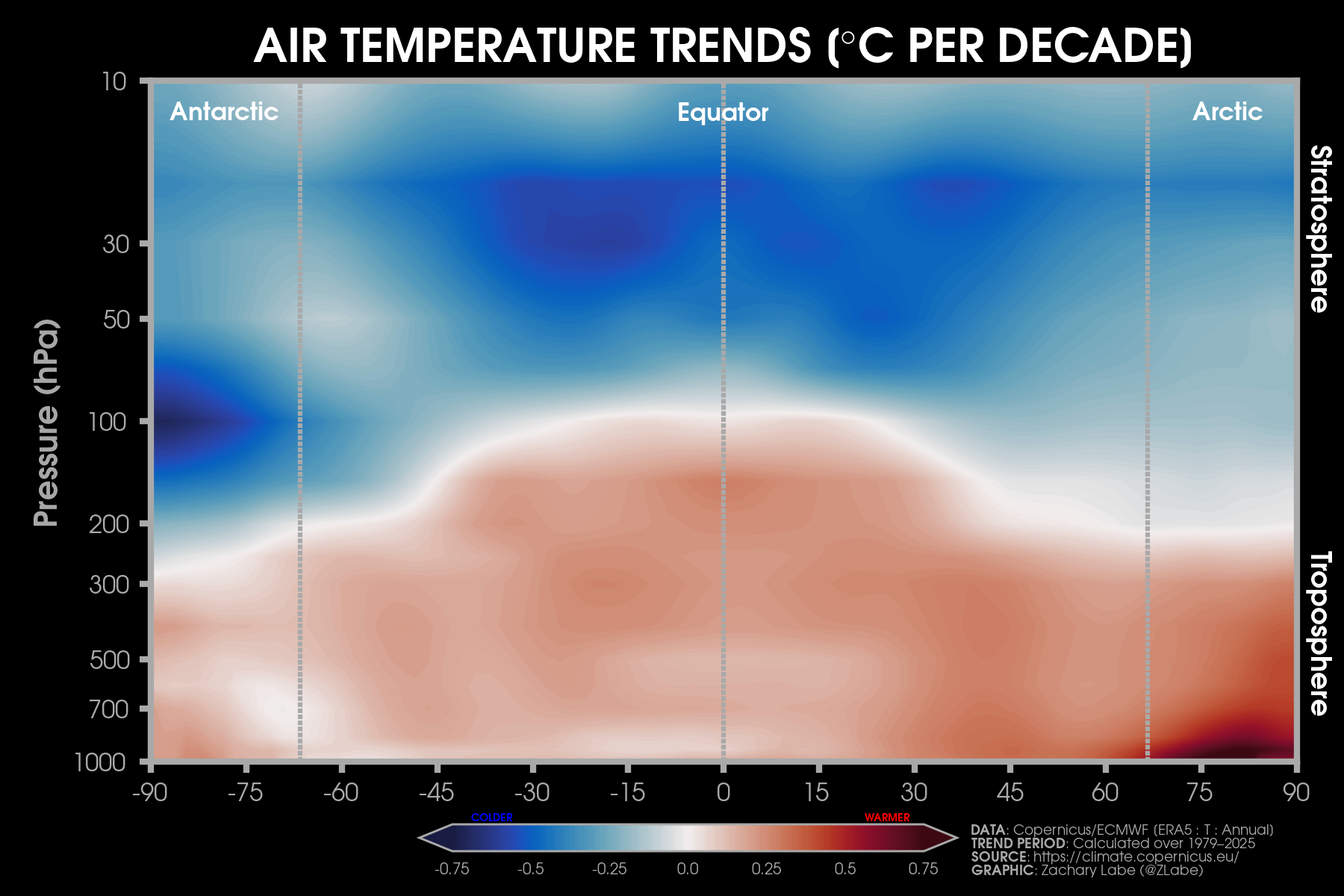
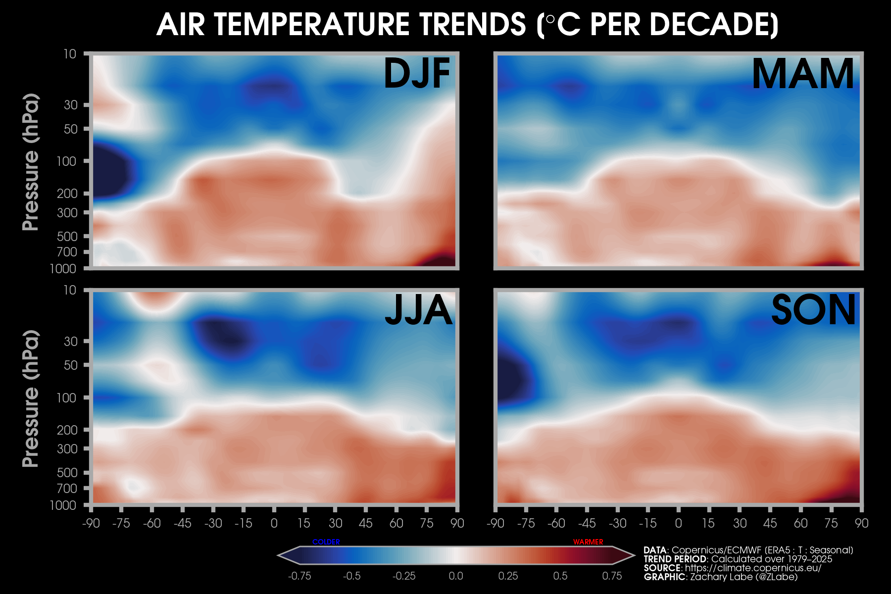
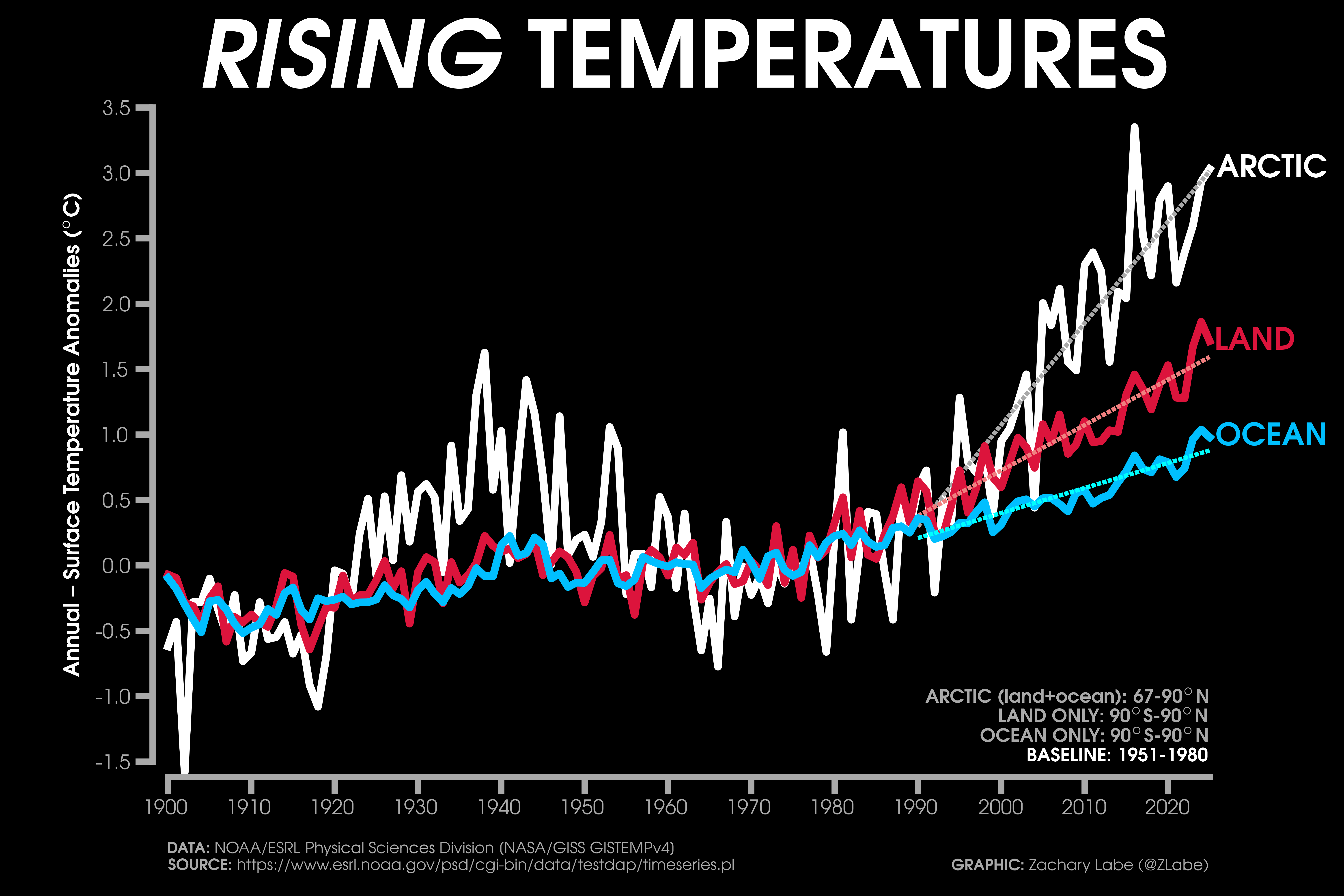
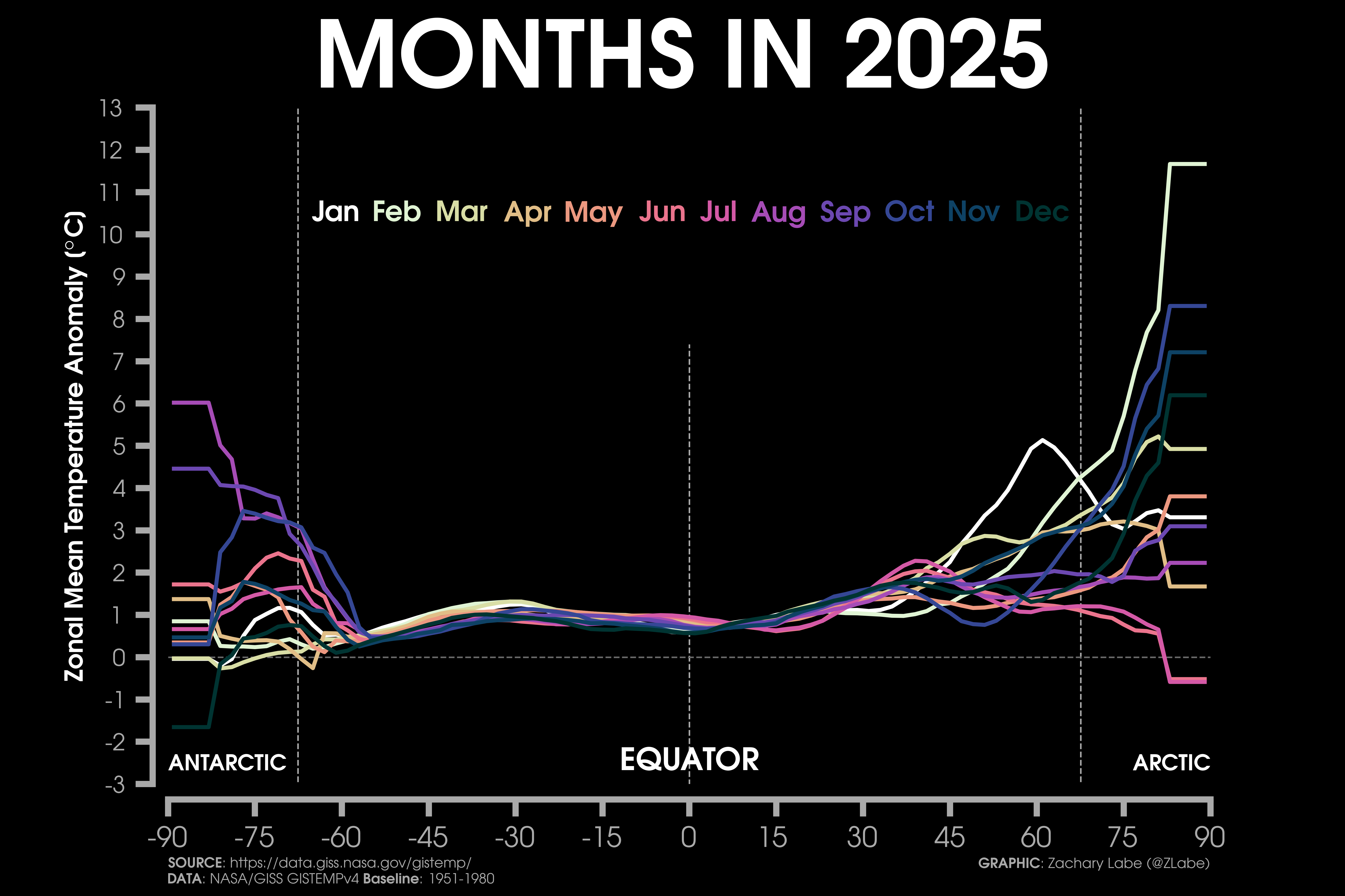
The views presented here only reflect my own. These figures may be freely distributed (with credit). Information about the data can be found on my references page and methods page.